Fractal nature of GD
Author: Umberto Michelucci
Version 1.0
import numpy as np
import pandas as pd
import matplotlib.pyplot as plt
import random
import matplotlib.patches as patches
Helper Functions
def sigma(z):
  return 1.0/(1+np.exp(-z))

# This function is not used in this notebook.
def generate_path_3(X, y, w1initial, w2initial, gamma_, iter):
  # The lists contain the initial values
  w1Path = [w1initial]
  w2Path = [w2initial]
  gamma = gamma_
  for i in range (iter): # Iterations

      j = random.randrange(3)

      w1_prev = w1Path[-1]
      w2_prev = w2Path[-1]

      s = X[j,0]*w1_prev+X[j,1]*w2_prev
      w1_new = w1_prev - gamma*(sigma(s)-y[j])*sigma(s)*(1-sigma(s))*X[j,0]
      #w1Path.append(w1_new)
      #w1_prev = w1Path[-1]

      w2_new = w2_prev - gamma*(sigma(s)-y[j])*sigma(s)*(1-sigma(s))*X[j,1]
      w2Path.append(w2_new)
      w1Path.append(w1_new)
  return np.array(w1Path), np.array(w2Path)


def generate_path_2(w1initial, w2initial, gamma_, iter):
  # The lists contain the initial values
  w1Path = [w1initial]
  w2Path = [w2initial]
  gamma = gamma_
  for i in range (iter): # Iterations

      j = random.randrange(3)

      w1_prev = w1Path[-1]
      w2_prev = w2Path[-1]

      w1_new = w1_prev - gamma*(X[j,0]*w1_prev+X[j,1]*w2_prev-y[j])*X[j,0]
      #w1Path.append(w1_new)
      #w1_prev = w1Path[-1]

      w2_new = w2_prev - gamma*(X[j,0]*w1_prev+X[j,1]*w2_prev-y[j])*X[j,1]
      w2Path.append(w2_new)
      w1Path.append(w1_new)
  return np.array(w1Path), np.array(w2Path)

# The following function has a different way of choosing randomly
# the observation. This version does not create the same fractal
# Structures.
def generate_path(w1initial, w2initial, gamma_, iter):
  # The lists contain the initial values
  w1Path = [w1initial]
  w2Path = [w2initial]
  gamma = gamma_
  for i in range (iter): # Iterations

    rand_sample = random.sample([0,1,2],3)
    #rand_sample = [0,1,2]
    for k in range (3): # the 3 input values
      j = rand_sample[k]

      w1_prev = w1Path[-1]
      w2_prev = w2Path[-1]

      w1_new = w1_prev - gamma*(X[j,0]*w1_prev+X[j,1]*w2_prev-y[j])*X[j,0]

      w2_new = w2_prev - gamma*(X[j,0]*w1_prev+X[j,1]*w2_prev-y[j])*X[j,1]
      w2Path.append(w2_new)
      w1Path.append(w1_new)
  return w1Path, w2Path
Data Preparation
We will use for this example 3 input observations, each having two features.
x1 = np.array([0,1])
x2 = np.array([1,0.5])
x3 = np.array([-1,0.5])

X = np.array([[0.0,1.0], [1.0,0.5], [1.0,-0.5]])
#X2 = np.array([[0.0,0.65], [0.45,0.57], [0.44,-0.32]])

y = np.array([0,4,0])
#y2 = np.array([0,0.7,0])
print(X)
print(y)
[[ 0.   1. ]
 [ 1.   0.5]
 [ 1.  -0.5]]
[0 4 0]
We will use a single neuron with an identity activation function. Meaning a neuron that generates a linear output
where \(x_{i1}\) and \(x_{i2}\) are the features of our \(i\) input observation.
For example (see the input matrix above) we will have \(x_{11}=0\) and \(x_{12}=1\). The loss function for one single observation \(l_i\) is
In this notebook we will use SGD, but we can follow two strategies in how we choose the sequence of observations to evaluate the weights update. In particular we can do the following
Ordered SGD (function: generate_path())
We choose a random order of the three observations. For example it could be 2,3,1
Then we evaluate the weight update by using, for each gradient calculations \(l_2\), \(l_3\) and finally \(l_1\)
We repeat the previous step a certain number of times.
Random SGD (function: generate_path2()
We simply choose each time a random observation and use it to udpate the weight.
3D Shape of Loss Function
Matrix Form
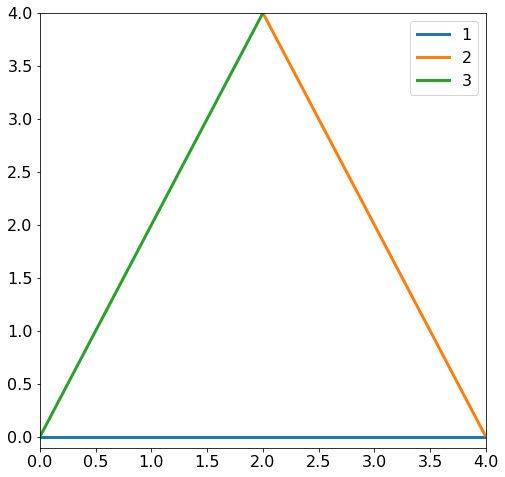
We can write the output of the network in matrix form (easily) as
where \(X\) and \(y\) are given above. The system above defines three lines in the parameter space \((w_1, w_2)\). If you are not convinced check that the matrix multiplication will give you three linear equations. The three lines defines a triangle that you can see in the figure below.
w1_ = np.arange(-1,4,0.01)
w2_1 = y[0]/X[0,1]-w1_/X[0,1]*X[0,0]
w2_2 = y[1]/X[1,1]-w1_/X[1,1]*X[1,0]
w2_3 = y[2]/X[2,1]-w1_/X[2,1]*X[2,0]
fig = plt.figure(figsize = (8,8))

plt.plot(w1_, w2_1, lw = 3, label = '1')
plt.plot(w1_, w2_2, lw = 3, label = '2')
plt.plot(w1_, w2_3, lw = 3, label = '3')
plt.legend(fontsize = 16)
plt.xticks(fontsize = 16)
plt.yticks(fontsize = 16)
plt.ylim(-.1, 4)
plt.xlim(0,4)
plt.show()
Minimum determination
We can use a couple of small tricks to determine the location of the minimum. This problem can also be solved by brute force by simply calcualting the derivatives of the total loss function
with respect to \(w_1\) and \(w_2\) and then solve the system.
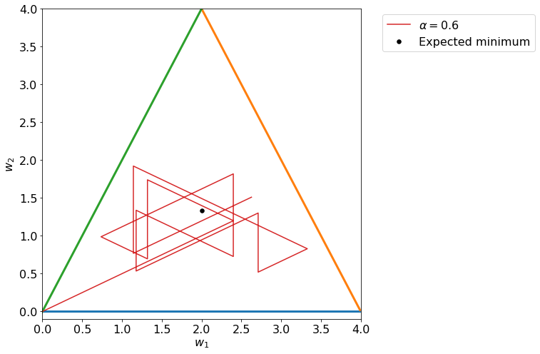
But we can be smarter. For example we can note that the slope of the line pependicular to a given line with a slope of \(m\) is \(-1/m\). Now let us take one of the lines we have defined above, for example the one with index \(i=2\):
This is the orange line in the figure above. Now let us suppose we use \(l_2\) for the weight updates. What do we get? Well we have
and
That means that the two weights updates will be
and
And you will notice easily that \(\Delta w_2 / \Delta w_1\) is nothing else that minus the inverse of the slope of the initial line. That means that the weight udpates when each observations is taken singularly goes along the perpendicular direction to the respective line.
fig = plt.figure(figsize = (8,8))

# Initial Point (0,0)
# Learning rate is 0.6
w1Path, w2Path = generate_path(0,0,0.6,5)

plt.plot(w1_, w2_1, lw = 3)
plt.plot(w1_, w2_2, lw = 3)
plt.plot(w1_, w2_3, lw = 3)
plt.legend()
plt.ylim(-0.1,4)
plt.xlim(0,4)


plt.xticks(fontsize = 16)
plt.yticks(fontsize = 16)
plt.xlabel('$w_1$', fontsize = 16)
plt.ylabel('$w_2$', fontsize = 16)
plt.plot(w1Path, w2Path,  label = r'$\alpha = 0.6$')
plt.scatter(2,4/3, marker = 'o', s = 30, color = 'black', zorder = 100, label = 'Expected minimum')

plt.legend(fontsize = 16, bbox_to_anchor=(1.05, 1))
plt.show()
No handles with labels found to put in legend.
The minimum can be found by symmetry. Note that given the symmetry of the lines, the minimum must be on the vertical line for \(w_1=2\). So the only thing we need to determine is the value of \(w_2\). So we can simply substitute \(w_1=2\) in the formula for \(L\)
derive it and set it equal to zero (remember we are looking for the minimum). We will get easily
This can be written (remember the values of \(X\) and \(y\)) as one single equation (we simply derive by \(w_2\)) as we know already \(w_1\):
this can be simplified as
that is $\( -2 + w_2 \frac{3}{2} = 0 \rightarrow w_2 = \frac{4}{3} \)$
So the minimum is located at \((2,\displaystyle\frac{4}{3})\).
Algorithm Convergence
Let us check now the set of points that we get by simply udpating weights one observation at a time in the same order (the initial order is determined randomlly, for example 2,3,1).
dist = 0.3
fig = plt.figure(figsize = (8,8))

ax = fig.add_subplot(1,1,1)

# Initial Point (0,0)
# Learning rate is
alpha = 0.1
w1Path, w2Path = generate_path(0,0,alpha,10**4)

plt.plot(w1_, w2_1, lw = 3)
plt.plot(w1_, w2_2, lw = 3)
plt.plot(w1_, w2_3, lw = 3)
plt.legend()
plt.ylim(-0.1,4)
plt.xlim(0,4)


plt.xticks(fontsize = 16)
plt.yticks(fontsize = 16)
plt.xlabel('$w_1$', fontsize = 16)
plt.ylabel('$w_2$', fontsize = 16)
plt.scatter(w1Path, w2Path,  label = r'$\alpha = $'+str(alpha), s = 5, color = 'cornflowerblue')
plt.scatter(2,4/3, marker = 'o', s = 30, color = 'black', zorder = 100, label = 'Expected minimum')

#rect = patches.Rectangle((2.0-dist, 4.0/3.0-dist), 2.0*dist, 2.0*dist, linewidth=3, edgecolor='black', facecolor='none', zorder = 200)
#ax.add_patch(rect)


# inset axes....
axins = ax.inset_axes([1.1, 0.25, 0.5, 0.5])
axins.scatter(w1Path, w2Path,  label = r'$\alpha = 0.1$', s = 5, color = 'cornflowerblue')
axins.plot(w1Path[5000:5010], w2Path[5000:5010],  label = r'$\alpha = 0.1$ (10 iter.)',  color = 'red')
axins.scatter(2,4/3, marker = 'o', s = 30, color = 'black', zorder = 100, label = 'Expected minimum')

# sub region of the original image
x1, x2, y1, y2 = 2.0-dist, 2.0+dist, 4.0/3.0-dist, 4.0/3.0+dist
axins.set_xlim(x1, x2)
axins.set_ylim(y1, y2)
axins.set_xticklabels('')
axins.set_yticklabels('')

ax.indicate_inset_zoom(axins, edgecolor="black", lw = 3, label = '')

plt.legend(fontsize = 16, bbox_to_anchor=(1.05, 1))

plt.show()
No handles with labels found to put in legend.
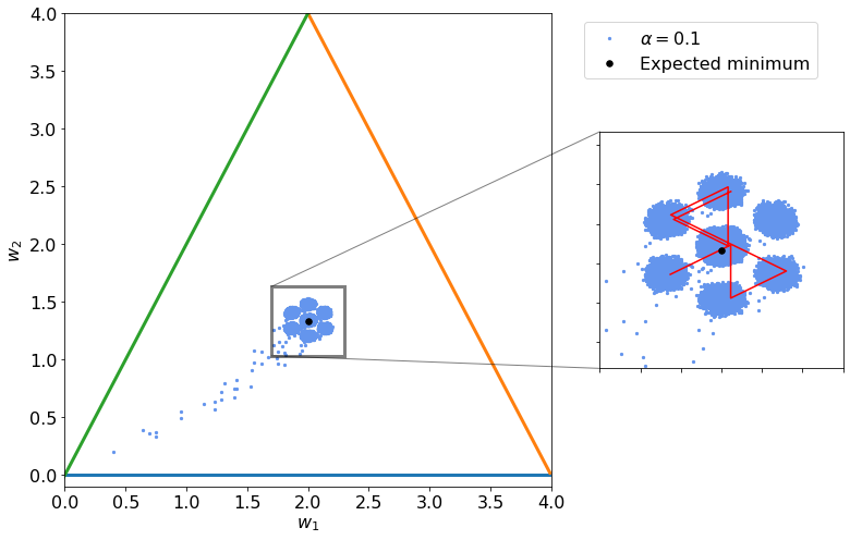
The algorithm does not really converges and simply oscillates around the minimum (indicated by the black dot).
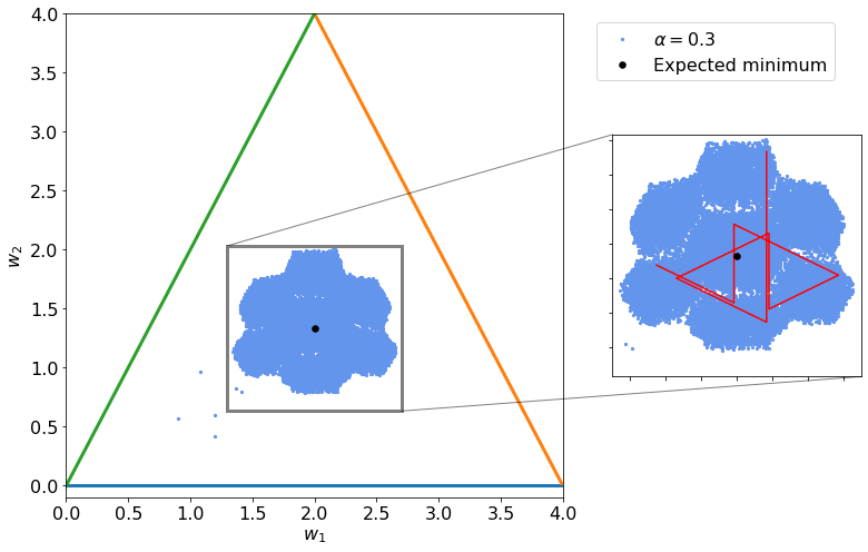
Below you can see another example with a larger value of \(\alpha = 0.3\).
dist = 0.7
fig = plt.figure(figsize = (8,8))

ax = fig.add_subplot(1,1,1)

# Initial Point (0,0)
# Learning rate is
alpha = 0.3
w1Path, w2Path = generate_path(0,0,alpha,10**4)

plt.plot(w1_, w2_1, lw = 3)
plt.plot(w1_, w2_2, lw = 3)
plt.plot(w1_, w2_3, lw = 3)
plt.legend()
plt.ylim(-0.1,4)
plt.xlim(0,4)


plt.xticks(fontsize = 16)
plt.yticks(fontsize = 16)
plt.xlabel('$w_1$', fontsize = 16)
plt.ylabel('$w_2$', fontsize = 16)
plt.scatter(w1Path, w2Path,  label = r'$\alpha = $'+str(alpha), s = 5, color = 'cornflowerblue')
plt.scatter(2,4/3, marker = 'o', s = 30, color = 'black', zorder = 100, label = 'Expected minimum')

# inset axes....
axins = ax.inset_axes([1.1, 0.25, 0.5, 0.5])
axins.scatter(w1Path, w2Path,  label = r'$\alpha = 0.1$', s = 5, color = 'cornflowerblue')
axins.plot(w1Path[5000:5010], w2Path[5000:5010],  label = r'$\alpha = 0.1$ (10 iter.)',  color = 'red')
axins.scatter(2,4/3, marker = 'o', s = 30, color = 'black', zorder = 100, label = 'Expected minimum')


# sub region of the original image
x1, x2, y1, y2 = 2.0-dist, 2.0+dist, 4.0/3.0-dist, 4.0/3.0+dist
axins.set_xlim(x1, x2)
axins.set_ylim(y1, y2)
axins.set_xticklabels('')
axins.set_yticklabels('')

ax.indicate_inset_zoom(axins, edgecolor="black", lw = 3, label = '')

plt.legend(fontsize = 16, bbox_to_anchor=(1.05, 1))

plt.show()
No handles with labels found to put in legend.
Gradients
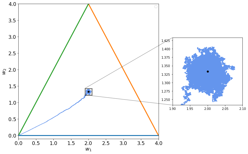
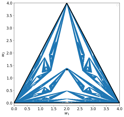
Now we can try to update the weights in a random manner (meaning not in the same order). This small change in how we update the weights disrupt completely the output of what happens in parameter space. You can see below what happens: Fractals appears!!
fig = plt.figure(figsize = (8,8))

# Initial Point (0,0)
# Learning rate is 0.6
w1Path, w2Path = generate_path_2(0,0,0.65,400000)

plt.plot(w1_, w2_1, lw = 3, color = 'black')
plt.plot(w1_, w2_2, lw = 3, color = 'black')
plt.plot(w1_, w2_3, lw = 3, color = 'black')
plt.legend()
plt.ylim(-0.1,4)
plt.xlim(0,4)


plt.xticks(fontsize = 16)
plt.yticks(fontsize = 16)
plt.xlabel('$w_1$', fontsize = 16)


plt.xticks(fontsize = 16)
plt.yticks(fontsize = 16)
plt.xlabel('$w_1$', fontsize = 16)
plt.ylabel('$w_2$', fontsize = 16)
plt.scatter(w1Path, w2Path,  label = r'$\alpha = 0.65$', s = 1)
plt.scatter(2,4/3, marker = 'o', s = 30, color = 'black', zorder = 100, label = 'Expected minimum')

#plt.legend(fontsize = 16, bbox_to_anchor=(1.05, 1))
#plt.ylabel('$w_2$', fontsize = 16)
#plt.scatter(w1Path, w2Path,  label = r'$\alpha = 0.65$')
#plt.scatter(2,4/3, marker = 'o', s = 30, color = 'black', zorder = 100, label = 'Expected minimum')

#plt.legend(fontsize = 16, bbox_to_anchor=(1.05, 1))
fig.savefig('fractal1.png', dpi = 300)
plt.show()
No handles with labels found to put in legend.
w1Path, w2Path = generate_path_2(0,0,0.65,10**7)
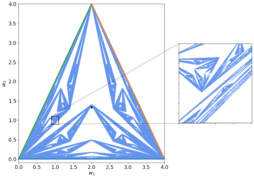
You can see below in the zommed out region that this is a fractal. The zoom looks exactly how the entire image! Note that this is not the definition of a fractal but is an amazing property of such structures!
dist = 0.7
fig = plt.figure(figsize = (14,8))

ax = fig.add_subplot(1,1,1)

# Initial Point (0,0)
# Learning rate is
alpha = 0.65
#w1Path, w2Path = generate_path(0,0,alpha,10**4)

plt.plot(w1_, w2_1, lw = 3)
plt.plot(w1_, w2_2, lw = 3)
plt.plot(w1_, w2_3, lw = 3)
plt.legend()
plt.ylim(-0.1,4)
plt.xlim(0,4)


plt.xticks(fontsize = 16)
plt.yticks(fontsize = 16)
plt.xlabel('$w_1$', fontsize = 16)
plt.ylabel('$w_2$', fontsize = 16)
plt.scatter(w1Path, w2Path,  label = r'$\alpha = $'+str(alpha), s = 0.5, color = 'cornflowerblue')
plt.scatter(2,4/3, marker = 'o', s = 30, color = 'black', zorder = 100, label = 'Expected minimum')

# inset axes....
axins = ax.inset_axes([1.1, 0.25, 0.5, 0.5])
axins.scatter(w1Path, w2Path,  label = r'$\alpha = 0.1$', s = 0.1, color = 'cornflowerblue')
axins.plot(w1Path[5000:5010], w2Path[5000:5010],  label = r'$\alpha = 0.65$ (10 iter.)',  color = 'red')
axins.scatter(2,4/3, marker = 'o', s = 30, color = 'black', zorder = 100, label = 'Expected minimum')


# sub region of the original image
x1, x2, y1, y2 = 0.9, 1.1, 0.9, 1.1
axins.set_xlim(x1, x2)
axins.set_ylim(y1, y2)
axins.set_xticklabels('')
axins.set_yticklabels('')

ax.indicate_inset_zoom(axins, edgecolor="black", lw = 3, label = '')

#plt.legend(fontsize = 16, bbox_to_anchor=(1.05, 1))
plt.tight_layout()
fig.savefig('fractl2.png', dpi = 300)
plt.show()
No handles with labels found to put in legend.
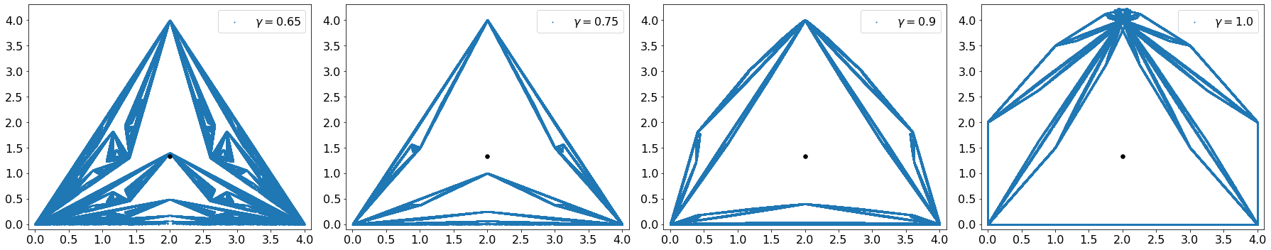
By changing the parameters you can see the differences in output and how the resulting structures change.
N = 10**6
fig = plt.figure(figsize = (25,5))

fig.add_subplot(1,4,1)
w1Path, w2Path = generate_path_2(0,0,0.65,N)

plt.legend()
plt.ylim(-0.1, 4.3)
plt.xlim(-0.1,4.1)

#plt.xlim(1.6, 2.4)
#plt.ylim(1.0,1.7)


plt.scatter(w1Path, w2Path, s = 1, label = '$\gamma = 0.65$')
plt.scatter(2,4/3, marker = 'o', s = 30, color = 'black', zorder = 100)

plt.legend(fontsize = 16)
plt.xticks(fontsize = 16)
plt.yticks(fontsize = 16)


fig.add_subplot(1,4,2)
w1Path, w2Path = generate_path_2(0,0,0.75,N)


plt.legend(fontsize = 16)
plt.ylim(-0.1, 4.3)
plt.xlim(-0.1,4.1)


plt.scatter(w1Path, w2Path, s = 1, label = '$\gamma = 0.75$')
plt.scatter(2,4/3, marker = 'o', s = 30, color = 'black', zorder = 100)

plt.legend(fontsize = 16)
plt.xticks(fontsize = 16)
plt.yticks(fontsize = 16)

fig.add_subplot(1,4,3)
w1Path, w2Path = generate_path_2(0,0,0.9,N)


plt.legend(fontsize = 16)
plt.ylim(-0.1, 4.3)
plt.xlim(-0.1,4.1)

#plt.xlim(1.6, 2.4)
#plt.ylim(1.0,1.7)


plt.scatter(w1Path, w2Path, s = 1, label = '$\gamma = 0.9$')
plt.scatter(2,4/3, marker = 'o', s = 30, color = 'black', zorder = 100)

plt.legend(fontsize = 16)
plt.xticks(fontsize = 16)
plt.yticks(fontsize = 16)

fig.add_subplot(1,4,4)
w1Path, w2Path = generate_path_2(0,0,1.0,N)


plt.ylim(-0.1, 4.3)
plt.xlim(-0.1,4.1)


#plt.xlim(1.6, 2.4)
#plt.ylim(1.0,1.7)


plt.scatter(w1Path, w2Path, s = 1, label = '$\gamma = 1.0$')
plt.scatter(2,4/3, marker = 'o', s = 30, color = 'black', zorder = 100)

plt.legend(fontsize = 16, loc = 'upper right')
plt.xticks(fontsize = 16)
plt.yticks(fontsize = 16)
plt.tight_layout()
fig.savefig('fractals3.png', dpi = 300)

plt.show()
No handles with labels found to put in legend.
No handles with labels found to put in legend.
No handles with labels found to put in legend.
N = 10**6
fig = plt.figure(figsize = (25,5))

fig.add_subplot(1,4,1)
w1Path, w2Path = generate_path_2(0,0,0.65,N)

plt.legend()
plt.ylim(-0.1, 4.3)
plt.xlim(-0.1,4.1)

#plt.xlim(1.6, 2.4)
#plt.ylim(1.0,1.7)


plt.scatter(w1Path, w2Path, s = 1, label = '$\gamma = 0.65$')
plt.scatter(2,4/3, marker = 'o', s = 30, color = 'black', zorder = 100)

plt.legend(fontsize = 16)
plt.xticks(fontsize = 16)
plt.yticks(fontsize = 16)


fig.add_subplot(1,4,2)
w1Path, w2Path = generate_path_2(0,0,0.5,N)


plt.legend(fontsize = 16)
plt.ylim(-0.1, 4.3)
plt.xlim(-0.1,4.1)


plt.scatter(w1Path, w2Path, s = 1, label = '$\gamma = 0.5$')
plt.scatter(2,4/3, marker = 'o', s = 30, color = 'black', zorder = 100)

plt.legend(fontsize = 16)
plt.xticks(fontsize = 16)
plt.yticks(fontsize = 16)

fig.add_subplot(1,4,3)
w1Path, w2Path = generate_path_2(0,0,0.3,N)


plt.legend(fontsize = 16)
plt.ylim(-0.1, 4.3)
plt.xlim(-0.1,4.1)

#plt.xlim(1.6, 2.4)
#plt.ylim(1.0,1.7)


plt.scatter(w1Path, w2Path, s = 1, label = '$\gamma = 0.3$')
plt.scatter(2,4/3, marker = 'o', s = 30, color = 'black', zorder = 100)

plt.legend(fontsize = 16)
plt.xticks(fontsize = 16)
plt.yticks(fontsize = 16)

fig.add_subplot(1,4,4)
w1Path, w2Path = generate_path_2(0,0,0.1,N)


plt.ylim(-0.1, 4.3)
plt.xlim(-0.1,4.1)


#plt.xlim(1.6, 2.4)
#plt.ylim(1.0,1.7)


plt.scatter(w1Path, w2Path, s = 1, label = '$\gamma = 0.1$')
plt.scatter(2,4/3, marker = 'o', s = 30, color = 'black', zorder = 100)

plt.legend(fontsize = 16, loc = 'upper right')
plt.xticks(fontsize = 16)
plt.yticks(fontsize = 16)
plt.tight_layout()

fig.savefig('fractals4.png', dpi = 300)

plt.show()
No handles with labels found to put in legend.
No handles with labels found to put in legend.
No handles with labels found to put in legend.
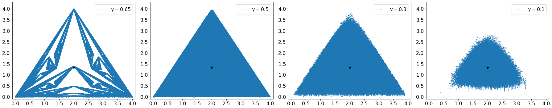
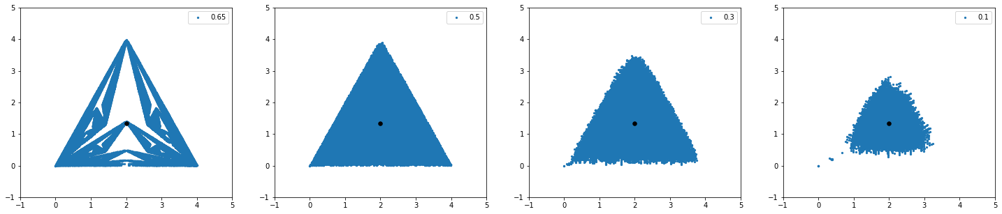
By reducing the parameter the fractal nature of the structure disappears suddenly and a cloud of points just appear as you can see in the images above and below.
N = 10**5
fig = plt.figure(figsize = (25,5))

fig.add_subplot(1,4,1)
w1Path, w2Path = generate_path_2(0,0,0.65,N)

plt.legend()
plt.ylim(-1, 5)
plt.xlim(-1,5)

#plt.xlim(1.6, 2.4)
#plt.ylim(1.0,1.7)


plt.scatter(w1Path, w2Path, s = 5, label = '0.65')
plt.scatter(2,4/3, marker = 'o', s = 30, color = 'black', zorder = 100)

plt.legend()


fig.add_subplot(1,4,2)
w1Path, w2Path = generate_path_2(0,0,0.5,N)


plt.legend()
plt.ylim(-1, 5)
plt.xlim(-1,5)

#plt.xlim(1.6, 2.4)
#plt.ylim(1.0,1.7)


plt.scatter(w1Path, w2Path, s = 5, label = '0.5')
plt.scatter(2,4/3, marker = 'o', s = 30, color = 'black', zorder = 100)

plt.legend()

fig.add_subplot(1,4,3)
w1Path, w2Path = generate_path_2(0,0,0.3,N)


plt.legend()
plt.ylim(-1, 5)
plt.xlim(-1,5)

#plt.xlim(1.6, 2.4)
#plt.ylim(1.0,1.7)


plt.scatter(w1Path, w2Path, s = 5, label = '0.3')
plt.scatter(2,4/3, marker = 'o', s = 30, color = 'black', zorder = 100)

plt.legend()


fig.add_subplot(1,4,4)
w1Path, w2Path = generate_path_2(0,0,0.1,N)


plt.ylim(-1, 5)
plt.xlim(-1,5)


#plt.xlim(1.6, 2.4)
#plt.ylim(1.0,1.7)


plt.scatter(w1Path, w2Path, s = 5, label = '0.1')
plt.scatter(2,4/3, marker = 'o', s = 30, color = 'black', zorder = 100)

plt.legend()

plt.show()
No handles with labels found to put in legend.
No handles with labels found to put in legend.
No handles with labels found to put in legend.
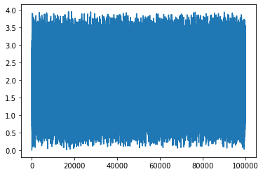
w1Path, w2Path = generate_path_2(0,0,0.5,N)
plt.plot(w1Path)
[<matplotlib.lines.Line2D at 0x7faa968a7650>]
w1Path, w2Path = generate_path_2(0,0,0.1,N)
plt.plot(w1Path)
[<matplotlib.lines.Line2D at 0x7faa96837890>]
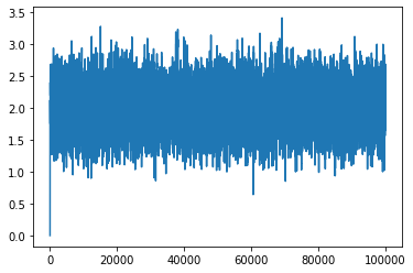
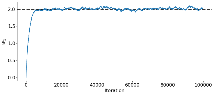
Evolution of parameters vs. Iteration Number
plt.figure(figsize = (12,5))
plt.xticks(fontsize = 16)
plt.yticks(fontsize = 16)
plt.xlabel('Iteration', fontsize = 16)
plt.ylabel('$w_1$', fontsize = 16)
w1Path, w2Path = generate_path_2(0,0,0.001,N)
plt.axhline(2.0, ls = '--', lw = 3, color = 'black')
plt.plot(w1Path)
[<matplotlib.lines.Line2D at 0x7faa968ff6d0>]
alpha = 0.0005
w1Path, w2Path = generate_path_2(0,0,alpha,N)
dist = 0.1
fig = plt.figure(figsize = (14,7))

ax = fig.add_subplot(1,1,1)

# Initial Point (0,0)
# Learning rate is
#alpha = 0.3
#w1Path, w2Path = generate_path(0,0,alpha,10**4)

plt.plot(w1_, w2_1, lw = 3)
plt.plot(w1_, w2_2, lw = 3)
plt.plot(w1_, w2_3, lw = 3)
plt.legend()
plt.ylim(-0.1,4)
plt.xlim(0,4)


plt.xticks(fontsize = 16)
plt.yticks(fontsize = 16)
plt.xlabel('$w_1$', fontsize = 16)
plt.ylabel('$w_2$', fontsize = 16)
plt.plot(w1Path, w2Path,  label = r'$\alpha = $'+str(alpha),  color = 'cornflowerblue')
plt.scatter(2,4/3, marker = 'o', s = 30, color = 'black', zorder = 100, label = 'Expected minimum')

# inset axes....
axins = ax.inset_axes([1.1, 0.25, 0.5, 0.5])
axins.plot(w1Path, w2Path,  label = r'$\alpha = 0.1$', color = 'cornflowerblue')
axins.plot(w1Path[5000:5010], w2Path[5000:5010],  label = r'$\alpha = 0.1$ (10 iter.)',  color = 'red')
axins.scatter(2,4/3, marker = 'o', s = 30, color = 'black', zorder = 100, label = 'Expected minimum')


# sub region of the original image
x1, x2, y1, y2 = 2.0-dist, 2.0+dist, 4.0/3.0-dist, 4.0/3.0+dist
axins.set_xlim(x1, x2)
axins.set_ylim(y1, y2)
#axins.set_xticklabels('')
#axins.set_yticklabels('')

ax.indicate_inset_zoom(axins, edgecolor="black", lw = 3, label = '')

#plt.legend(fontsize = 16, bbox_to_anchor=(1.05, 1))

plt.tight_layout()
fig.savefig('fractals5.png', dpi = 300)
plt.show()
No handles with labels found to put in legend.