.ipynb .pdf

repository open issue

Binder Colab

Contents

Regularization Techniques

Version 1.0

(C) 2020 - Umberto Michelucci, Michela Sperti

This notebook is part of the book Applied Deep Learning: a case based approach, 2nd edition from APRESS by U. Michelucci and M. Sperti.

The purpose of this notebook is to show you an example of extreme overfitting in the case of a linear regression model applied to a dataset taken from the real world. Then a series of strategies are presented (called regularization techniques) which can help us try to solve this issue, without the need of changing the network’s architecture or the model itself.

Notebook Learning Goals

At the end of this notebook you will clearly know what overfitting is and how to treat it by means of regularization and dropout techniques. In particular you will know how to implement in Keras \(L_2\) and \(L_1\) regularization techniques, dropout and early stopping.

Libraries and Dataset Import

This section contains the necessary libraries (such as tensorflow or pandas) you need to import to run the notebook.

# general libraries
import numpy as np
import pandas as pd
import matplotlib.pyplot as plt
import matplotlib.font_manager as fm

# tensorflow libraries
import tensorflow as tf
from tensorflow import keras
from tensorflow.keras import layers

# sklearn libraries
from sklearn.datasets import load_boston

# Referring to the following cell, if you want to re-clone a repository
# inside the google colab instance, you need to delete it first. 
# You can delete the repositories contained in this instance executing 
# the following two lines of code (deleting the # comment symbol).

# !rm -rf ADL-Book-2nd-Ed 

# This command actually clone the repository of the book in the google colab
# instance. In this way this notebook will have access to the modules
# we have written for this book.

# Please note that in case you have already run this cell, and you run it again
# you may get the error message:
#
# fatal: destination path 'ADL-Book-2nd-Ed' already exists and is not an empty directory.
# 
# In this case you can safely ignore the error message.

!git clone https://github.com/toelt-llc/ADL-Book-2nd-Ed.git

Cloning into 'ADL-Book-2nd-Ed'...
remote: Enumerating objects: 237, done.
remote: Counting objects: 100% (237/237), done.
remote: Compressing objects: 100% (193/193), done.
remote: Total 1164 (delta 61), reused 199 (delta 44), pack-reused 927
Receiving objects: 100% (1164/1164), 180.25 MiB | 25.74 MiB/s, done.
Resolving deltas: 100% (489/489), done.

# This cell imports some custom written functions that we have created to 
# make the plotting easier. You don't need to undertsand the details and 
# you can simply ignore this cell.
# Simply run it with CMD+Enter (on Mac) or CTRL+Enter (Windows or Ubuntu) to
# import the necessary functions.

import sys
sys.path.append('ADL-Book-2nd-Ed/modules/')

from style_setting import set_style

In this notebook we will use the Boston dataset. Check the Further Readings section to have more details about this dataset. It is very straightforward to import, by means of scikit-learn library, which already contains the dataset, ready to be used. The following cells are needed to automatically download the dataset and have it in the notebook.

boston = load_boston()
features = np.array(boston.data)
target = np.array(boston.target)

Let’s have a look at the description of the Boston dataset.

print(boston['DESCR'])

.. _boston_dataset:

Boston house prices dataset
---------------------------

**Data Set Characteristics:**  

    :Number of Instances: 506 

    :Number of Attributes: 13 numeric/categorical predictive. Median Value (attribute 14) is usually the target.

    :Attribute Information (in order):
        - CRIM     per capita crime rate by town
        - ZN       proportion of residential land zoned for lots over 25,000 sq.ft.
        - INDUS    proportion of non-retail business acres per town
        - CHAS     Charles River dummy variable (= 1 if tract bounds river; 0 otherwise)
        - NOX      nitric oxides concentration (parts per 10 million)
        - RM       average number of rooms per dwelling
        - AGE      proportion of owner-occupied units built prior to 1940
        - DIS      weighted distances to five Boston employment centres
        - RAD      index of accessibility to radial highways
        - TAX      full-value property-tax rate per $10,000
        - PTRATIO  pupil-teacher ratio by town
        - B        1000(Bk - 0.63)^2 where Bk is the proportion of blacks by town
        - LSTAT    % lower status of the population
        - MEDV     Median value of owner-occupied homes in $1000's

    :Missing Attribute Values: None

    :Creator: Harrison, D. and Rubinfeld, D.L.

This is a copy of UCI ML housing dataset.
https://archive.ics.uci.edu/ml/machine-learning-databases/housing/


This dataset was taken from the StatLib library which is maintained at Carnegie Mellon University.

The Boston house-price data of Harrison, D. and Rubinfeld, D.L. 'Hedonic
prices and the demand for clean air', J. Environ. Economics & Management,
vol.5, 81-102, 1978.   Used in Belsley, Kuh & Welsch, 'Regression diagnostics
...', Wiley, 1980.   N.B. Various transformations are used in the table on
pages 244-261 of the latter.

The Boston house-price data has been used in many machine learning papers that address regression
problems.   
     
.. topic:: References

   - Belsley, Kuh & Welsch, 'Regression diagnostics: Identifying Influential Data and Sources of Collinearity', Wiley, 1980. 244-261.
   - Quinlan,R. (1993). Combining Instance-Based and Model-Based Learning. In Proceedings on the Tenth International Conference of Machine Learning, 236-243, University of Massachusetts, Amherst. Morgan Kaufmann.

Let’s get the dimension of the data set now.

n_training_samples = features.shape[0]
n_dim = features.shape[1]

print('The dataset has', n_training_samples, 'training samples.')
print('The dataset has', n_dim, 'features.')

The dataset has 506 training samples.
The dataset has 13 features.

So, in the variable n_training_samples we have the number of different input observations, and in the variable n_dim we have the number of features (or variables if you like) that we have at our disposal.

Dataset Normalization

The following function is needed to normalize the different features, since this helps learning. As you can see, this is done by means of NumPy wonderful vectorized code.

def normalize(dataset):
    mu = np.mean(dataset, axis = 0)
    sigma = np.std(dataset, axis = 0)
    return (dataset - mu)/sigma

features_norm = normalize(features)

Extreme Overfitting

Now we will use the Boston dataset to go into a situation of extreme ovefitting. We will apply a linear regression model performed by means of deep neural networks to the Boston dataset. If you don’t remember the details of linear regression implemented with deep neural networks you can check Linear_regression_with_one_neuron.ipynb notebook, in Chapter 14.

First of all, we split our dataset into training (80% of the original dataset) and dev (20% of the original dataset) sets.

np.random.seed(42)
rnd = np.random.rand(len(features_norm)) < 0.8

train_x = features_norm[rnd]
train_y = target[rnd]
dev_x = features_norm[~rnd]
dev_y = target[~rnd]

print(train_x.shape)
print(train_y.shape)
print(dev_x.shape)
print(dev_y.shape)

(399, 13)
(399,)
(107, 13)
(107,)

Let’s look at what happens when we try to do linear regression with a network with 4 layers with 20 neurons each.

The following function builds and trains a feed-forward neural network model for linear regression and evaluates it on the training and dev sets. If you don’t remember what a feed-forward neural network is, you can check the Multiclass_classification_with_fully_connected_networks.ipynb notebook in Chapter 15.

def create_and_train_model_nlayers(data_train_norm, labels_train, data_dev_norm, labels_dev, num_neurons, num_layers):
    # build model
    inputs = keras.Input(shape = data_train_norm.shape[1]) # input layer
    # he initialization
    initializer = tf.keras.initializers.HeNormal()
    # first hidden layer
    dense = layers.Dense(num_neurons, activation = 'relu', kernel_initializer = initializer)(inputs)
    # customized number of layers and neurons per layer
    for i in range(num_layers - 1):       
        dense = layers.Dense(num_neurons, activation = 'relu', kernel_initializer = initializer)(dense)
    # output layer   
    outputs = layers.Dense(1)(dense)
    model = keras.Model(inputs = inputs, outputs = outputs, name = 'model')
    # set optimizer and loss
    opt = keras.optimizers.Adam(learning_rate = 0.001)
    model.compile(loss = 'mse', optimizer = opt, metrics = ['mse'])
    
    # train model
    history = model.fit(
      data_train_norm, labels_train,
      epochs = 10000, verbose = 0,
      batch_size = data_train_norm.shape[0],
      validation_data = (data_dev_norm, labels_dev))
    # save performances
    hist = pd.DataFrame(history.history)
    hist['epoch'] = history.epoch 

    return hist, model

hist, model = create_and_train_model_nlayers(train_x, train_y, dev_x, dev_y, 20, 4)

Now we want to plot the dev vs training mean square error (MSE) to understand if we are in overfitting regime.

Cost Function on the Training and Dev Dataset Plot

# The following line contains the path to fonts that are used to plot result in
# a uniform way.

f = set_style().set_general_style_parameters()

# Cost Function vs. Number of Iterations plot for training and dev datasets

fig = plt.figure()
ax = fig.add_subplot(111)

ax.plot(hist['loss'], ls = '-', color = 'black', lw = 3, label = 'Training MSE')
ax.plot(hist['val_loss'], ls = '--', color = 'blue', lw = 2, label = 'Dev MSE')
plt.ylabel('Cost Function (MSE)', fontproperties = fm.FontProperties(fname = f))
plt.xlabel('Number of Iterations', fontproperties = fm.FontProperties(fname = f))
ax.set_ylim(0, 30)
plt.legend(loc = 'best')

plt.axis(True)
#plt.savefig('./Figure16-1.png', dpi = 300)
plt.show()

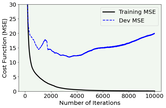
As you can see from the above plot, we are in a situation of extreme overfitting. In fact, while the error on the training dataset quickly reaches the zero, the error on the dev dataset reaches a value of 15 and then it starts increasing until a value of 20. This means that our model has learnt useless features of the training dataset (for example noise) and that it cannot generalize on newly unseen data samples.

Another easy way of checking how our regression model is working is to plot the predicted values vs. the true values for both the training and dev datasets. If our regression would be perfect, all the points would be placed on the diagonal, if not they would spread around it.

# predictions
pred_y_train = model.predict(train_x).flatten()
pred_y_dev = model.predict(dev_x).flatten()

Predicted Values vs. True Values on Training and Dev Dataset Plot

# predicted values vs. true values plot for training and dev datasets

fig = plt.figure(figsize = (13, 5))
ax = fig.add_subplot(121)

ax.scatter(train_y, pred_y_train, s = 50, color = 'blue', label = 'MSE Training = ' + '{:5.4f}'.format(hist['loss'].values[-1]))
ax.plot([np.min(np.array(dev_y)), np.max(np.array(dev_y))], [np.min(np.array(dev_y)), np.max(np.array(dev_y))], 'k--', lw = 3)
ax.set_xlabel('Measured Target Value', fontproperties = fm.FontProperties(fname = f))
ax.set_ylabel('Predicted Target Value', fontproperties = fm.FontProperties(fname = f))
ax.set_ylim(0, 55)
ax.legend(loc = 'best')

ax = fig.add_subplot(122)
ax.scatter(dev_y, pred_y_dev, s = 50, color = 'blue', label = 'MSE Dev = ' + '{:5.2f}'.format(hist['val_loss'].values[-1]))
ax.plot([np.min(np.array(dev_y)), np.max(np.array(dev_y))], [np.min(np.array(dev_y)), np.max(np.array(dev_y))], 'k--', lw = 3)
ax.set_xlabel('Measured Target Value', fontproperties = fm.FontProperties(fname = f))
ax.set_ylim(0, 55)
ax.legend(loc = 'best')

plt.axis(True)
#plt.savefig('./Figure16-2.png', dpi = 300)
plt.show()

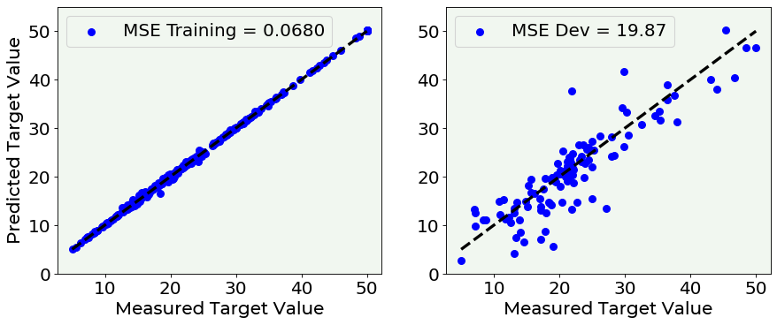
And, as expected, the model behaves perfectly on the training dataset and poorly on the dev dataset. In the left plot all the points stand on the diagonal line, with a very low MSE, while in the right plot the points are more scattered and the MSE increases. This means that the predictions on the dev test are quite different from the target labels.

So, the natural question now is: why does the model go into overfitting regime? How to avoid it? The answer to the first question is quite easy and it is linked to the complexity of our network: too many layers and too many neurons learn useless information from the training dataset.

Concerning the second question, there are many ways to try to reduce overfitting. The most straightforward is to reduce the complexity of the network. However, this is a very time-consuming process, mostly when we have very big datasets which require time to be trained. In fact we have to try different architecture and decide which is the right one.

An alternative solution to the problem of overfitting is regularization. Let us see more in detail how to perform it.

Regularization

We are now going to try a regularization method to deal with the problem of overfitting.

First of all, it is important to know that the concept of regularization in machine learning has a long history, starting from the 90s, and evolving over time. If you are interest in different views on what regularization means, check the Further Readings section of the notebook.

In this notebook, we will consider regularization as a way to try to avoid overfitting. More specifically, this is achieved by reducing the number of network’s weights which are not zero, during the training phase.

We will start from \({\bf L_2}\) regularization technique, which consists of adding a term to the cost function with the aim of reducing the effective capacity of the network to adapt to complex datasets.

\(L_2\) Regularization Technique

Applying \(L_2\) regularization technique, the cost function is defined as follow

\[ \tilde{J}({\bf w})={J({\bf w})+\frac{\lambda}{2m}{||{\bf w}||}^2}_2 \]

where \({\frac{\lambda}{2m}{||{\bf w}||}^2}_2\) is called the regularization term (\(m\) is the number of observations) and \(\lambda\) is called the regularization parameter.

We will define \(\lambda\) in Keras as an additional hyper-parameter and we will search for its optimal value (i.e. the one that prevents the network from going into overfitting regime).

Notice that in Keras the \(L_2\) regularization penalty is computed as: loss = l2 * reduce_sum(square(x)).

def create_and_train_reg_model_L2(data_train_norm, labels_train, data_dev_norm, labels_dev, num_neurons, num_layers, n_epochs, lambda_):
    # build model
    inputs = keras.Input(shape = data_train_norm.shape[1]) # input layer
    # he initialization
    initializer = tf.keras.initializers.HeNormal()
    # regularization
    reg = tf.keras.regularizers.l2(l2 = lambda_)
    # first hidden layer
    dense = layers.Dense(num_neurons, activation = 'relu', kernel_initializer = initializer, kernel_regularizer = reg)(inputs)
    # customized number of layers and neurons per layer
    for i in range(num_layers - 1):       
        dense = layers.Dense(num_neurons, activation = 'relu', kernel_initializer = initializer, kernel_regularizer = reg)(dense)
    # output layer   
    outputs = layers.Dense(1)(dense)
    model = keras.Model(inputs = inputs, outputs = outputs, name = 'model')
    # set optimizer and loss
    opt = keras.optimizers.Adam(learning_rate = 0.001)
    model.compile(loss = 'mse', optimizer = opt, metrics = ['mse'])
    
    # train model
    history = model.fit(
      data_train_norm, labels_train,
      epochs = n_epochs, verbose = 0,
      batch_size = data_train_norm.shape[0],
      validation_data = (data_dev_norm, labels_dev))
    # save performances
    hist = pd.DataFrame(history.history)
    hist['epoch'] = history.epoch 
    # print performances
    print('Cost function at epoch 0')
    print('Training MSE = ', hist['loss'].values[0])
    print('Dev MSE = ', hist['val_loss'].values[0])
    print('Cost function at epoch ' + str(n_epochs))
    print('Training MSE = ', hist['loss'].values[-1])
    print('Dev MSE = ', hist['val_loss'].values[-1])

    return hist, model

Number of Weights that are Zero

Let us evaluate and compare a situation in which the network is not regularized (\(\lambda = 0.0\)) and a situation in which we apply a regularization (\(\lambda = 10.0\)), printing on the screen the final loss function value in the case of the training and dev dataset.

\(\lambda = 0.0\) vs \(\lambda = 10.0\), \(5000\) epochs

hist_notreg, model_notreg = create_and_train_reg_model_L2(train_x, train_y, dev_x, dev_y, 20, 4, 5000, 0.0)

Cost function at epoch 0
Training MSE =  437.77789306640625
Dev MSE =  409.2901611328125
Cost function at epoch 5000
Training MSE =  0.3108246922492981
Dev MSE =  18.21949005126953

hist_reg, model_reg = create_and_train_reg_model_L2(train_x, train_y, dev_x, dev_y, 20, 4, 5000, 10.0)

Cost function at epoch 0
Training MSE =  2099.23779296875
Dev MSE =  2067.65234375
Cost function at epoch 5000
Training MSE =  54.47111511230469
Dev MSE =  53.30109786987305

As we said before, \(L_2\) regularization reduces the number of network’s weights which are not zero, during the training phase, and prevent the overfitting situation (in fact, as you can see, the MSE on the training and test after 5000 epochs are quite similar). Let us inspect how the weights have changed after regularization.

Let us first check how many weights have been reduced to zero during the regularization process.

The following lines extract the weights associated to each hidden layer in the case of the regularized version of the network and the not regularized one.

# not regularized network
weights1_notreg = model_notreg.layers[1].get_weights()[0]
weights2_notreg = model_notreg.layers[2].get_weights()[0]
weights3_notreg = model_notreg.layers[3].get_weights()[0]
weights4_notreg = model_notreg.layers[4].get_weights()[0]

# regularized network
weights1_reg = model_reg.layers[1].get_weights()[0]
weights2_reg = model_reg.layers[2].get_weights()[0]
weights3_reg = model_reg.layers[3].get_weights()[0]
weights4_reg = model_reg.layers[4].get_weights()[0]

Now we print the percentage of weights equal to zero inside each hidden layer.

print('NOT REGULARIZED NETWORK')
print('First hidden layer:')
print('{:.2f}'.format((np.sum(np.abs(weights1_notreg) < 1e-3)) / weights1_notreg.size * 100.0))
print('Second hidden layer:')
print('{:.2f}'.format((np.sum(np.abs(weights2_notreg) < 1e-3)) / weights2_notreg.size * 100.0))
print('Third hidden layer:')
print('{:.2f}'.format((np.sum(np.abs(weights3_notreg) < 1e-3)) / weights3_notreg.size * 100.0))
print('Fourth hidden layer:')
print('{:.2f}'.format((np.sum(np.abs(weights4_notreg) < 1e-3)) / weights4_notreg.size * 100.0))

NOT REGULARIZED NETWORK
First hidden layer:
0.38
Second hidden layer:
0.00
Third hidden layer:
0.25
Fourth hidden layer:
0.25

print('REGULARIZED NETWORK')
print('First hidden layer:')
print('{:.2f}'.format((np.sum(np.abs(weights1_reg) < 1e-3)) / weights1_reg.size * 100.0))
print('Second hidden layer:')
print('{:.2f}'.format((np.sum(np.abs(weights2_reg) < 1e-3)) / weights2_reg.size * 100.0))
print('Third hidden layer:')
print('{:.2f}'.format((np.sum(np.abs(weights3_reg) < 1e-3)) / weights3_reg.size * 100.0))
print('Fourth hidden layer:')
print('{:.2f}'.format((np.sum(np.abs(weights4_reg) < 1e-3)) / weights4_reg.size * 100.0))

REGULARIZED NETWORK
First hidden layer:
10.00
Second hidden layer:
37.75
Third hidden layer:
65.50
Fourth hidden layer:
64.25

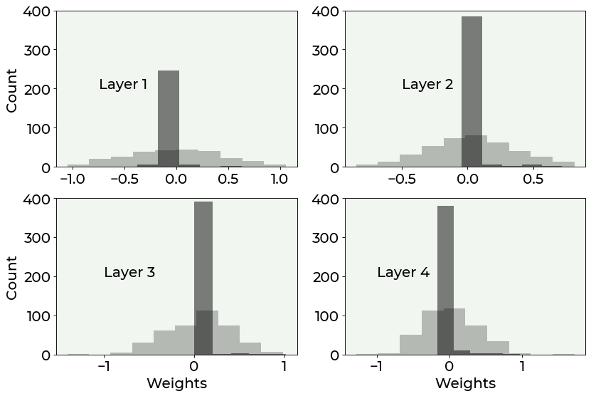
We can then compare the histogram of the weights with and without regularization (to have a more intuitive representation of the weights). The difference is quite stunning.

fig = plt.figure(figsize = (12, 8))
ax = fig.add_subplot(221)
plt.hist(weights1_notreg.flatten(), alpha = 0.25, bins = 10, color = 'black')
plt.hist(weights1_reg.flatten(), alpha = 0.5, bins = 5, color = 'black')
ax.set_ylabel('Count', fontproperties = fm.FontProperties(fname = f))
ax.text(-1, 150, 'Layer 1', fontproperties = fm.FontProperties(fname = f))
plt.xticks(fontproperties = fm.FontProperties(fname = f))
plt.yticks(fontproperties = fm.FontProperties(fname = f)) 
plt.ylim(0, 350)

ax = fig.add_subplot(222)
plt.hist(weights2_notreg.flatten(), alpha = 0.25, bins = 10, color = 'black')
plt.hist(weights2_reg.flatten(), alpha = 0.5, bins = 5, color = 'black')
ax.text(-1.25, 150, 'Layer 2', fontproperties = fm.FontProperties(fname = f))
plt.xticks(fontproperties = fm.FontProperties(fname = f))
plt.yticks(fontproperties = fm.FontProperties(fname = f)) 
plt.ylim(0, 350)

ax = fig.add_subplot(223)
plt.hist(weights3_notreg.flatten(), alpha = 0.25, bins = 10, color = 'black')
plt.hist(weights3_reg.flatten(), alpha = 0.5, bins = 5, color = 'black')
ax.set_ylabel('Count', fontproperties = fm.FontProperties(fname = f))
ax.set_xlabel('Weights', fontproperties = fm.FontProperties(fname = f))
ax.text(-2.30, 150, 'Layer 3', fontproperties = fm.FontProperties(fname = f))
plt.xticks(fontproperties = fm.FontProperties(fname = f))
plt.yticks(fontproperties = fm.FontProperties(fname = f)) 
plt.ylim(0, 400)

ax = fig.add_subplot(224)
plt.hist(weights4_notreg.flatten(), alpha = 0.25, bins = 10, color = 'black')
plt.hist(weights4_reg.flatten(), alpha = 0.5, bins = 5, color = 'black')
ax.set_xlabel('Weights', fontproperties = fm.FontProperties(fname = f))
ax.text(-2.30, 150, 'Layer 4', fontproperties = fm.FontProperties(fname = f))
plt.xticks(fontproperties = fm.FontProperties(fname = f))
plt.yticks(fontproperties = fm.FontProperties(fname = f)) 
plt.ylim(0, 400)

#plt.savefig('./Figure16-3.png', dpi = 300)
plt.show()

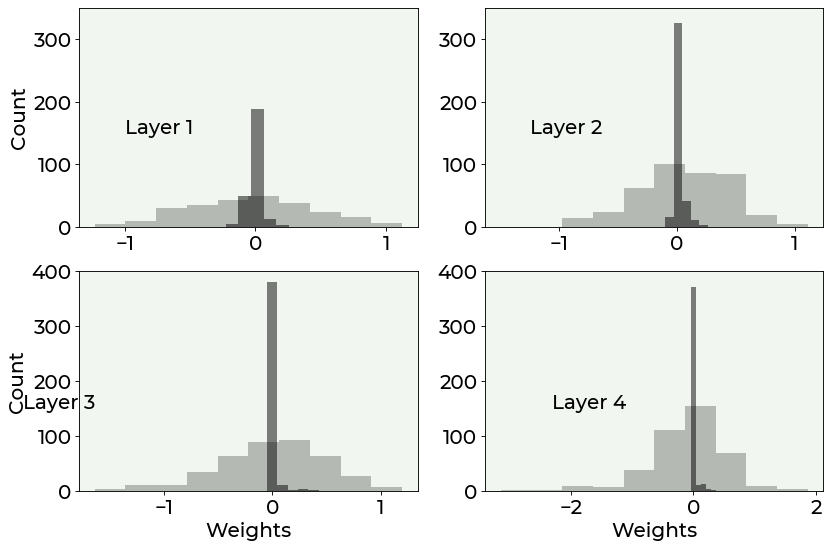
As you can see from the above plot, regularization effectively increases the number of weights which are zero, reducing overfitting by making the network simpler, without the need to change its architecture.

\(\lambda = 0.0\) vs \(\lambda = 3.0\), \(1000\) epochs

Let us inspect another case, comparing a not regularized network with a regularized one, with \(\lambda = 3.0\) and after 1000 epochs.

hist_notreg, model_notreg = create_and_train_reg_model_L2(train_x, train_y, dev_x, dev_y, 20, 4, 1000, 0.0)

Cost function at epoch 0
Training MSE =  588.55859375
Dev MSE =  561.6209106445312
Cost function at epoch 1000
Training MSE =  3.4968719482421875
Dev MSE =  20.51352310180664

hist_reg, model_reg = create_and_train_reg_model_L2(train_x, train_y, dev_x, dev_y, 20, 4, 1000, 3.0)

Cost function at epoch 0
Training MSE =  1022.06396484375
Dev MSE =  995.086181640625
Cost function at epoch 1000
Training MSE =  52.672828674316406
Dev MSE =  55.371116638183594

# not regularized network
weights1_notreg = model_notreg.layers[1].get_weights()[0]
weights2_notreg = model_notreg.layers[2].get_weights()[0]
weights3_notreg = model_notreg.layers[3].get_weights()[0]
weights4_notreg = model_notreg.layers[4].get_weights()[0]

# regularized network
weights1_reg = model_reg.layers[1].get_weights()[0]
weights2_reg = model_reg.layers[2].get_weights()[0]
weights3_reg = model_reg.layers[3].get_weights()[0]
weights4_reg = model_reg.layers[4].get_weights()[0]

print('NOT REGULARIZED NETWORK')
print('First hidden layer:')
print('{:.2f}'.format((np.sum(np.abs(weights1_notreg) < 1e-3)) / weights1_notreg.size * 100.0))
print('Second hidden layer:')
print('{:.2f}'.format((np.sum(np.abs(weights2_notreg) < 1e-3)) / weights2_notreg.size * 100.0))
print('Third hidden layer:')
print('{:.2f}'.format((np.sum(np.abs(weights3_notreg) < 1e-3)) / weights3_notreg.size * 100.0))
print('Fourth hidden layer:')
print('{:.2f}'.format((np.sum(np.abs(weights4_notreg) < 1e-3)) / weights4_notreg.size * 100.0))

NOT REGULARIZED NETWORK
First hidden layer:
0.77
Second hidden layer:
0.00
Third hidden layer:
1.00
Fourth hidden layer:
0.25

print('REGULARIZED NETWORK')
print('First hidden layer:')
print('{:.2f}'.format((np.sum(np.abs(weights1_reg) < 1e-3)) / weights1_reg.size * 100.0))
print('Second hidden layer:')
print('{:.2f}'.format((np.sum(np.abs(weights2_reg) < 1e-3)) / weights2_reg.size * 100.0))
print('Third hidden layer:')
print('{:.2f}'.format((np.sum(np.abs(weights3_reg) < 1e-3)) / weights3_reg.size * 100.0))
print('Fourth hidden layer:')
print('{:.2f}'.format((np.sum(np.abs(weights4_reg) < 1e-3)) / weights4_reg.size * 100.0))

REGULARIZED NETWORK
First hidden layer:
1.54
Second hidden layer:
28.25
Third hidden layer:
40.00
Fourth hidden layer:
45.75

Training and Dev MSE vs. \(\lambda\) Plot

How can we choose \(\lambda\)? A very useful tip may be to plot the behaviour of the MSE on the training and dev sets, given a specific network, for many \(\lambda\) parameters.

Let us calculate the performances:

train_mse, dev_mse = [], []
lambda_values = [0.0, 2.5, 5.0, 7.5, 10.0, 12.5, 15.0, 17.5, 20.0]

for lambda_ in lambda_values:
  
  print('Lambda = ', lambda_)
  hist_, model_ = create_and_train_reg_model_L2(train_x, train_y, dev_x, dev_y, 20, 4, 1000, lambda_)
  train_mse.append(hist_['loss'].values[-1])
  dev_mse.append(hist_['val_loss'].values[-1])
  print()

Lambda =  0.0
Cost function at epoch 0
Training MSE =  651.7122192382812
Dev MSE =  615.8396606445312
Cost function at epoch 1000
Training MSE =  3.743802547454834
Dev MSE =  16.33320426940918

Lambda =  2.5
Cost function at epoch 0
Training MSE =  989.0043334960938
Dev MSE =  960.2646484375
Cost function at epoch 1000
Training MSE =  48.386962890625
Dev MSE =  51.39109802246094

Lambda =  5.0
Cost function at epoch 0
Training MSE =  1516.9046630859375
Dev MSE =  1480.40478515625
Cost function at epoch 1000
Training MSE =  62.484893798828125
Dev MSE =  63.04401397705078

Lambda =  7.5
Cost function at epoch 0
Training MSE =  1772.639892578125
Dev MSE =  1738.387939453125
Cost function at epoch 1000
Training MSE =  73.22252655029297
Dev MSE =  71.78938293457031

Lambda =  10.0
Cost function at epoch 0
Training MSE =  2200.84375
Dev MSE =  2164.82763671875
Cost function at epoch 1000
Training MSE =  89.33045196533203
Dev MSE =  85.83134460449219

Lambda =  12.5
Cost function at epoch 0
Training MSE =  2630.42333984375
Dev MSE =  2593.941650390625
Cost function at epoch 1000
Training MSE =  103.18284606933594
Dev MSE =  98.20773315429688

Lambda =  15.0
Cost function at epoch 0
Training MSE =  3095.466064453125
Dev MSE =  3055.00927734375
Cost function at epoch 1000
Training MSE =  118.67585754394531
Dev MSE =  112.77542114257812

Lambda =  17.5
Cost function at epoch 0
Training MSE =  3383.120849609375
Dev MSE =  3345.5634765625
Cost function at epoch 1000
Training MSE =  118.77632904052734
Dev MSE =  112.03402709960938

Lambda =  20.0
Cost function at epoch 0
Training MSE =  3794.609375
Dev MSE =  3753.96435546875
Cost function at epoch 1000
Training MSE =  127.06510162353516
Dev MSE =  119.71223449707031

And let us plot the final result.

fig = plt.figure()
ax = fig.add_subplot(111)

ax.plot(lambda_values, train_mse, ls = '-', color = 'black', lw = 3, label = 'Training MSE')
ax.plot(lambda_values, dev_mse, ls = '--', color = 'blue', lw = 2, label = 'Dev MSE')
plt.ylabel('Cost Function (MSE)', fontproperties = fm.FontProperties(fname = f))
plt.xlabel('$\lambda$', fontproperties = fm.FontProperties(fname = f))
ax.set_xticks(lambda_values)
plt.legend(loc = 'best')

plt.axis(True)
#plt.savefig('./Figure16-4.png', dpi = 300)
plt.show()

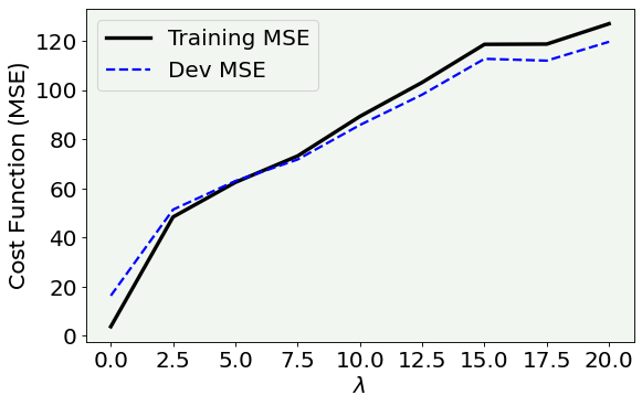
As you can see, a good choice for the \(\lambda\) parameter in this specific case (always remember that in the deep learning world there is no a unique rule) may be 6, since in this point the MSE on the training and on the dev datasets are almost the same. Before 6 in the plot, the model tends to overfit the data (since the error on the training is higher than the error on the dev set), while after 6 the model becomes too simple and cannot capture the main features of the dataset.

\(L_1\) Regularization Technique

As for \(L_2\) regularization, the implementation in Keras is straightforward.

\({\bf L_1}\) regularization also works by adding an additional term to the cost function:

\[ \tilde{J}({\bf w})={J({\bf w})+\frac{\lambda}{m}{||{\bf w}||}}_1 \]

As before, we will define \(\lambda\) in Keras as an additional hyper-parameter and we will search for its optimal value (i.e. the one that prevents the network from going into overfitting regime).

Notice that in Keras the \(L_1\) regularization penalty is computed as: loss = l1 * reduce_sum(abs(x)).

def create_and_train_reg_model_L1(data_train_norm, labels_train, data_dev_norm, labels_dev, num_neurons, num_layers, n_epochs, lambda_):
    # build model
    inputs = keras.Input(shape = data_train_norm.shape[1]) # input layer
    # he initialization
    initializer = tf.keras.initializers.HeNormal()
    # regularization
    reg = tf.keras.regularizers.l1(l1 = lambda_)
    # first hidden layer
    dense = layers.Dense(num_neurons, activation = 'relu', kernel_initializer = initializer, kernel_regularizer = reg)(inputs)
    # customized number of layers and neurons per layer
    for i in range(num_layers - 1):       
        dense = layers.Dense(num_neurons, activation = 'relu', kernel_initializer = initializer, kernel_regularizer = reg)(dense)
    # output layer   
    outputs = layers.Dense(1)(dense)
    model = keras.Model(inputs = inputs, outputs = outputs, name = 'model')
    # set optimizer and loss
    opt = keras.optimizers.Adam(learning_rate = 0.001)
    model.compile(loss = 'mse', optimizer = opt, metrics = ['mse'])
    
    # train model
    history = model.fit(
      data_train_norm, labels_train,
      epochs = n_epochs, verbose = 0,
      batch_size = data_train_norm.shape[0],
      validation_data = (data_dev_norm, labels_dev))
    # save performances
    hist = pd.DataFrame(history.history)
    hist['epoch'] = history.epoch 
    # print performances
    print('Cost function at epoch 0')
    print('Training MSE = ', hist['loss'].values[0])
    print('Dev MSE = ', hist['val_loss'].values[0])
    print('Cost function at epoch ' + str(n_epochs))
    print('Training MSE = ', hist['loss'].values[-1])
    print('Dev MSE = ', hist['val_loss'].values[-1])

    return hist, model

The only change with respect to the function we wrote for implementing \(L_2\) regularizer is in the definition of the regularizer itself. Very simple!!!

Number of Weights that are Zero

Let us evaluate and compare a situation in which the network is not regularized (\(\lambda = 0.0\)) and a situation in which we apply a regularization (\(\lambda = 3.0\)), printing on the screen the final loss function value in the case of the training and dev dataset.

\(\lambda = 0.0\) vs \(\lambda = 3.0\), \(1000\) epochs

hist_notreg, model_notreg = create_and_train_reg_model_L1(train_x, train_y, dev_x, dev_y, 20, 4, 1000, 0.0)

Cost function at epoch 0
Training MSE =  582.0275268554688
Dev MSE =  555.6217651367188
Cost function at epoch 1000
Training MSE =  5.341501235961914
Dev MSE =  25.19839096069336

hist_reg, model_reg = create_and_train_reg_model_L1(train_x, train_y, dev_x, dev_y, 20, 4, 1000, 3.0)

Cost function at epoch 0
Training MSE =  1811.86376953125
Dev MSE =  1778.408447265625
Cost function at epoch 1000
Training MSE =  91.37516021728516
Dev MSE =  92.39669799804688

As expected, also \(L_1\) regularization effectively deals with overfitting (by reducing the difference between the training and dev set performances).

Let us inspect how many weights are close to zero, like we did for \(L_2\) regularizer.

# not regularized network
weights1_notreg = model_notreg.layers[1].get_weights()[0]
weights2_notreg = model_notreg.layers[2].get_weights()[0]
weights3_notreg = model_notreg.layers[3].get_weights()[0]
weights4_notreg = model_notreg.layers[4].get_weights()[0]

# regularized network
weights1_reg = model_reg.layers[1].get_weights()[0]
weights2_reg = model_reg.layers[2].get_weights()[0]
weights3_reg = model_reg.layers[3].get_weights()[0]
weights4_reg = model_reg.layers[4].get_weights()[0]

print('NOT REGULARIZED NETWORK')
print('First hidden layer:')
print('{:.2f}'.format((np.sum(np.abs(weights1_notreg) < 1e-3)) / weights1_notreg.size * 100.0))
print('Second hidden layer:')
print('{:.2f}'.format((np.sum(np.abs(weights2_notreg) < 1e-3)) / weights2_notreg.size * 100.0))
print('Third hidden layer:')
print('{:.2f}'.format((np.sum(np.abs(weights3_notreg) < 1e-3)) / weights3_notreg.size * 100.0))
print('Fourth hidden layer:')
print('{:.2f}'.format((np.sum(np.abs(weights4_notreg) < 1e-3)) / weights4_notreg.size * 100.0))

NOT REGULARIZED NETWORK
First hidden layer:
0.00
Second hidden layer:
0.50
Third hidden layer:
0.00
Fourth hidden layer:
0.00

print('REGULARIZED NETWORK')
print('First hidden layer:')
print('{:.2f}'.format((np.sum(np.abs(weights1_reg) < 1e-3)) / weights1_reg.size * 100.0))
print('Second hidden layer:')
print('{:.2f}'.format((np.sum(np.abs(weights2_reg) < 1e-3)) / weights2_reg.size * 100.0))
print('Third hidden layer:')
print('{:.2f}'.format((np.sum(np.abs(weights3_reg) < 1e-3)) / weights3_reg.size * 100.0))
print('Fourth hidden layer:')
print('{:.2f}'.format((np.sum(np.abs(weights4_reg) < 1e-3)) / weights4_reg.size * 100.0))

REGULARIZED NETWORK
First hidden layer:
90.77
Second hidden layer:
94.50
Third hidden layer:
96.75
Fourth hidden layer:
94.50

fig = plt.figure(figsize = (12, 8))
ax = fig.add_subplot(221)
plt.hist(weights1_notreg.flatten(), alpha = 0.25, bins = 10, color = 'black')
plt.hist(weights1_reg.flatten(), alpha = 0.5, bins = 5, color = 'black')
ax.set_ylabel('Count', fontproperties = fm.FontProperties(fname = f))
ax.text(-0.75, 200, 'Layer 1', fontproperties = fm.FontProperties(fname = f))
plt.xticks(fontproperties = fm.FontProperties(fname = f))
plt.yticks(fontproperties = fm.FontProperties(fname = f)) 
plt.ylim(0, 400)

ax = fig.add_subplot(222)
plt.hist(weights2_notreg.flatten(), alpha = 0.25, bins = 10, color = 'black')
plt.hist(weights2_reg.flatten(), alpha = 0.5, bins = 5, color = 'black')
ax.text(-0.5, 200, 'Layer 2', fontproperties = fm.FontProperties(fname = f))
plt.xticks(fontproperties = fm.FontProperties(fname = f))
plt.yticks(fontproperties = fm.FontProperties(fname = f)) 
plt.ylim(0, 400)

ax = fig.add_subplot(223)
plt.hist(weights3_notreg.flatten(), alpha = 0.25, bins = 10, color = 'black')
plt.hist(weights3_reg.flatten(), alpha = 0.5, bins = 5, color = 'black')
ax.set_ylabel('Count', fontproperties = fm.FontProperties(fname = f))
ax.set_xlabel('Weights', fontproperties = fm.FontProperties(fname = f))
ax.text(-1, 200, 'Layer 3', fontproperties = fm.FontProperties(fname = f))
plt.xticks(fontproperties = fm.FontProperties(fname = f))
plt.yticks(fontproperties = fm.FontProperties(fname = f)) 
plt.ylim(0, 400)

ax = fig.add_subplot(224)
plt.hist(weights4_notreg.flatten(), alpha = 0.25, bins = 10, color = 'black')
plt.hist(weights4_reg.flatten(), alpha = 0.5, bins = 5, color = 'black')
ax.set_xlabel('Weights', fontproperties = fm.FontProperties(fname = f))
ax.text(-1, 200, 'Layer 4', fontproperties = fm.FontProperties(fname = f))
plt.xticks(fontproperties = fm.FontProperties(fname = f))
plt.yticks(fontproperties = fm.FontProperties(fname = f)) 
plt.ylim(0, 400)

#plt.savefig('./Figure16-8.png', dpi = 300)
plt.show()

Are the weights really going to zero?

We are now using a simulated dataset to visually see how fast the weights of a regularized deep neural network goes to zero.

nobs = 30 # number of observations
np.random.seed(42) # making results reproducible

# first set of observations
xx1 = np.array([np.random.normal(0.3, 0.15) for i in range (0, nobs)])
yy1 = np.array([np.random.normal(0.3, 0.15) for i in range (0, nobs)])
# second set of observations
xx2 = np.array([np.random.normal(0.1, 0.1) for i in range (0, nobs)])
yy2 = np.array([np.random.normal(0.3, 0.1) for i in range (0, nobs)])
# concatenating observations
c1_ = np.c_[xx1.ravel(), yy1.ravel()]
c2_ = np.c_[xx2.ravel(), yy2.ravel()] 
c = np.concatenate([c1_, c2_])
# creating the labels
yy1_ = np.full(nobs, 0, dtype = int)
yy2_ = np.full(nobs, 1, dtype = int)
yyL = np.concatenate((yy1_, yy2_), axis = 0)
# defining training points and labels
train_x = c
train_y = yyL

Our dataset has two features: \(x\) and \(y\). Two group of points have been generated from a normal distribution:

• (xx1, yy1), of class 0

• (xx2, yy2), of class 1

We will follow the behaviour of a specific weight (\(w_{12,5}^{[3]}\) from layer 3) along the 1000 epochs. The network has been \(L_2\)-regularized (\(\lambda=0.1\)).

To get weights for every epoch from a Keras model it is necessary to use a callback function. We are not going into the details of callback functions here, since they are widely explained in another Chapter, specifically dedicated to them. The only thing you need to know now is that Keras does not automatically save each weight’s value during training. To have them, we need to use callbacks.

With the following code we train the model for binary classification and we save the weights for each epoch.

weights_dict = {}
weight_history = []

# build model
inputs = keras.Input(shape = train_x.shape[1]) # input layer
# he initialization
initializer = tf.keras.initializers.HeNormal()
# regularization
reg = tf.keras.regularizers.l2(l2 = 0.1)
# hidden layers
dense = layers.Dense(20, activation = 'relu', kernel_initializer = initializer, kernel_regularizer = reg)(inputs)
dense = layers.Dense(20, activation = 'relu', kernel_initializer = initializer, kernel_regularizer = reg)(dense)
dense = layers.Dense(20, activation = 'relu', kernel_initializer = initializer, kernel_regularizer = reg)(dense)
dense = layers.Dense(20, activation = 'relu', kernel_initializer = initializer, kernel_regularizer = reg)(dense)    
# output layer   
outputs = layers.Dense(1, activation = 'sigmoid')(dense)
model = keras.Model(inputs = inputs, outputs = outputs, name = 'model')
# set optimizer and loss
opt = keras.optimizers.Adam(learning_rate = 0.001)
model.compile(loss = 'binary_crossentropy', optimizer = opt, metrics = ['accuracy'])
# set callback function
weight_callback = tf.keras.callbacks.LambdaCallback(on_epoch_end = lambda epoch, logs: weights_dict.update({epoch: model.get_weights()}))
# train model
history = model.fit(
  train_x, train_y,
  epochs = 1000, verbose = 0,
  batch_size = train_x.shape[0],
  callbacks = weight_callback)

We then keep the values of the specific weight we are interested in.

# retrieve weights
for epoch, weights in weights_dict.items():
  weight_history.append(weights[6][5][12])

Finally we plot the weight’s decay rate.

# Weight's value vs. number of epoch plot
fig = plt.figure()
ax = fig.add_subplot(111)

ax.plot(weight_history, color = 'blue')
plt.ylabel('$w^{[3]}_{12,5}$', fontproperties = fm.FontProperties(fname = f))
plt.xlabel('Epochs', fontproperties = fm.FontProperties(fname = f))
ax.text(400, 0.08, 'Value after 1000 epochs:\n$1\cdot 10^{-16}$', fontproperties = fm.FontProperties(fname = f))

#plt.savefig('./Figure16-9.png', dpi = 300)
plt.show()

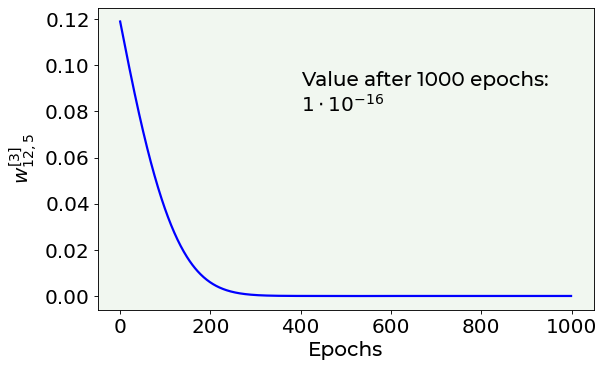
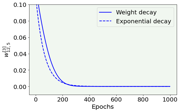
As you can notice, the weights really go down to zero and also very fast. How fast? Exponentially. Let us prove it visually, by comparing the above plot with an exponential decay.

# Weight's value vs. number of epoch plot compared to exponential decay
fig = plt.figure()
ax = fig.add_subplot(111)

ax.plot(weight_history, ls = '-', color = 'blue', label = 'Weight decay')
ax.plot(0.11 * np.exp(-np.arange(0, 1000, 1) / 63), ls = '--', color = 'blue', label = 'Exponential decay')
plt.ylabel('$w^{[3]}_{12,5}$', fontproperties = fm.FontProperties(fname = f))
plt.xlabel('Epochs', fontproperties = fm.FontProperties(fname = f))
plt.ylim(-0.01, 0.1)
plt.legend(loc = 'best')

#plt.savefig('./Figure16-10.png', dpi = 300)
plt.show()

Dropout

Another regularization technique is called dropout and its basic idea is the following: during the training phase of a deep neural network, nodes are removed randomly (with a specified probability \(p^{[l]}\)) from layer \(l\).

In Keras, you simply add how many dropout layers as you want after the layer you want to drop, with the following function: keras.layers.Dropout(rate).

In the above function you must put as input the layer you want to drop and you must set the rate parameter. This parameter can assume float values in the following range: \([0, 1)\), since it represents the fraction of the input units to drop. Therefore, it is not possible to drop all the units (setting a rate equal to 1).

Now, let us compare the results when applying or not dropout to the Boston dataset.

def create_and_train_reg_model_dropout(data_train_norm, labels_train, data_dev_norm, labels_dev, num_neurons, num_layers, n_epochs, rate):
    # build model
    inputs = keras.Input(shape = data_train_norm.shape[1]) # input layer
    # he initialization
    initializer = tf.keras.initializers.HeNormal()
    # first hidden layer
    dense = layers.Dense(num_neurons, activation = 'relu', kernel_initializer = initializer)(inputs)
    # first dropout layer
    dense = keras.layers.Dropout(rate)(dense)
    # customized number of layers and neurons per layer
    for i in range(num_layers - 1):   
        dense = layers.Dense(num_neurons, activation = 'relu', kernel_initializer = initializer)(dense)
        # customized number of dropout layers  
        dense = keras.layers.Dropout(rate)(dense)
    # output layer   
    outputs = layers.Dense(1)(dense)
    model = keras.Model(inputs = inputs, outputs = outputs, name = 'model')
    # set optimizer and loss
    opt = keras.optimizers.Adam(learning_rate = 0.001)
    model.compile(loss = 'mse', optimizer = opt, metrics = ['mse'])
    
    # train model
    history = model.fit(
      data_train_norm, labels_train,
      epochs = n_epochs, verbose = 0,
      batch_size = data_train_norm.shape[0],
      validation_data = (data_dev_norm, labels_dev))
    # save performances
    hist = pd.DataFrame(history.history)
    hist['epoch'] = history.epoch 
    # print performances
    print('Cost function at epoch 0')
    print('Training MSE = ', hist['loss'].values[0])
    print('Dev MSE = ', hist['val_loss'].values[0])
    print('Cost function at epoch ' + str(n_epochs))
    print('Training MSE = ', hist['loss'].values[-1])
    print('Dev MSE = ', hist['val_loss'].values[-1])

    return hist, model

hist_notreg, model_notreg = create_and_train_reg_model_dropout(train_x, train_y, dev_x, dev_y, 20, 4, 8000, 0.0)

Cost function at epoch 0
Training MSE =  617.59765625
Dev MSE =  587.8325805664062
Cost function at epoch 8000
Training MSE =  0.07932430505752563
Dev MSE =  16.718381881713867

hist_reg, model_reg = create_and_train_reg_model_dropout(train_x, train_y, dev_x, dev_y, 20, 4, 8000, 0.50)

Cost function at epoch 0
Training MSE =  729.6145629882812
Dev MSE =  649.31689453125
Cost function at epoch 8000
Training MSE =  53.04020309448242
Dev MSE =  54.92367935180664

In the following plot you can see the training dataset cost function vs. the number of epoch in the case of a model without regularization and another one with a dropout rate of 0.50.

# Cost function vs. number of epoch plot for a model trained with dropout and another one trained without dropout

fig = plt.figure()
ax = fig.add_subplot(111)

ax.plot(hist_notreg['loss'], color = 'blue', label = 'Without Dropout')
ax.plot(hist_reg['loss'], color = 'red', label = 'With Dropout')
plt.ylabel('Cost Function (MSE)', fontproperties = fm.FontProperties(fname = f))
plt.xlabel('Number of Iterations', fontproperties = fm.FontProperties(fname = f))
ax.set_xlim(0, 2000)
ax.set_ylim(0, 500)
plt.legend(loc = 'best')

plt.axis(True)
#plt.savefig('./Figure16-11.png', dpi = 300)
plt.show()

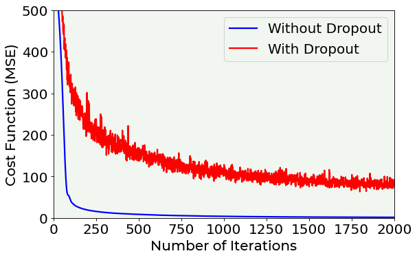
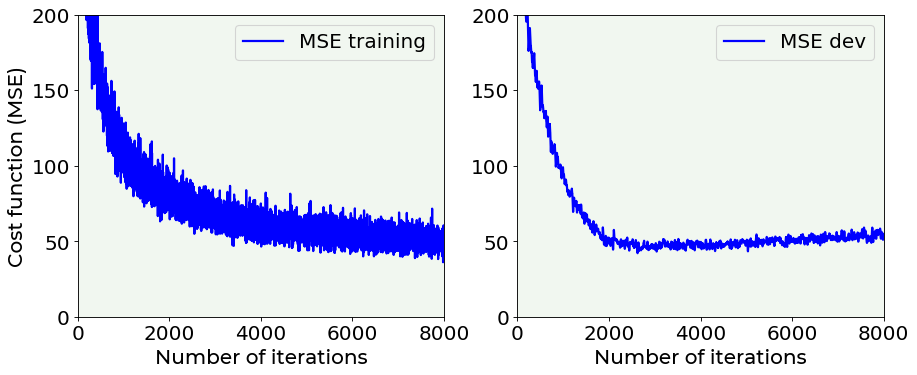
As you can see, when applying dropout, the cost function is very irregular. Let us now plot the cost function on the training and dev datasets, comparing them both when applying dropout and when not.

# cost function vs. number of epochs plot for training and dev datasets
# with dropout

fig = plt.figure(figsize = (13, 5))
ax = fig.add_subplot(121)

ax.plot(hist_reg['loss'], color = 'blue', label = 'MSE training')
ax.set_xlabel('Number of iterations', fontproperties = fm.FontProperties(fname = f))
ax.set_ylabel('Cost function (MSE)', fontproperties = fm.FontProperties(fname = f))
ax.set_xlim(0, 8000)
ax.set_ylim(0, 200)
ax.legend(loc = 'best')

ax = fig.add_subplot(122)
ax.plot(hist_reg['val_loss'], color = 'blue', label = 'MSE dev')
ax.set_xlabel('Number of iterations', fontproperties = fm.FontProperties(fname = f))
ax.set_xlim(0, 8000)
ax.set_ylim(0, 200)
ax.legend(loc = 'best')

plt.axis(True)
#plt.savefig('./Figure16-12.png', dpi = 300)
plt.show()

# cost function vs. number of epochs plot for training and dev datasets
# without dropout

fig = plt.figure(figsize = (13, 5))
ax = fig.add_subplot(121)

ax.plot(hist_notreg['loss'], color = 'blue', label = 'MSE training')
ax.set_xlabel('Number of iterations', fontproperties = fm.FontProperties(fname = f))
ax.set_ylabel('Cost function (MSE)', fontproperties = fm.FontProperties(fname = f))
ax.set_xlim(0, 8000)
ax.set_ylim(0, 40)
ax.legend(loc = 'best')

ax = fig.add_subplot(122)
ax.plot(hist_notreg['val_loss'], color = 'blue', label = 'MSE dev')
ax.set_xlabel('Number of iterations', fontproperties = fm.FontProperties(fname = f))
ax.set_xlim(0, 8000)
ax.set_ylim(0, 40)
ax.legend(loc = 'best')

plt.axis(True)
#plt.savefig('./Figure16-13.png', dpi = 300)
plt.show()

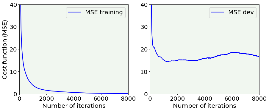
The difference between the two above plots is evident: it is very interesting the fact that without dropout \(MSE_{dev}\) grows with epochs, while using dropout it is rather stable. Without dropout, the model is in clear extreme overfitting regime, while with dropout you can see how the \(MSE_{train}\) and \(MSE_{dev}\) are of the same order of magnitude and the \(MSE_{dev}\) does not continue to grow, so we have a model that is a lot better at generalizing.

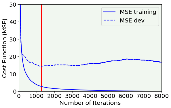
Early Stopping

Now the last technique that is sometime used to fight overfitting is early stopping. Strictly speaking this method does nothing to avoid overfitting, it simply stops the learning before the overfitting problem becomes too bad. In the above considered example, we can decide to stop the training phase when the \(MSE_{dev}\) reaches its minimum, as the red vertical line in the following plot indicates.

# Cost function vs. number of epoch plot for a model trained with dropout and another one trained without dropout

fig = plt.figure()
ax = fig.add_subplot(111)

ax.plot(hist_notreg['loss'], ls = '-', color = 'blue', label = 'MSE training')
ax.plot(hist_notreg['val_loss'], ls = '--', color = 'blue', label = 'MSE dev')
plt.vlines(np.argmin(hist_notreg['val_loss'].values), 0, 50, color = 'red')
plt.ylabel('Cost Function (MSE)', fontproperties = fm.FontProperties(fname = f))
plt.xlabel('Number of Iterations', fontproperties = fm.FontProperties(fname = f))
ax.set_xlim(0, 8000)
ax.set_ylim(0, 50)
plt.legend(loc = 'best')

plt.axis(True)
plt.savefig('./Figure16-14.png', dpi = 300)
plt.show()

Note that this is not an ideal way of solving the overfitting problem. Your model will still most probably generalize very badly to new data. It is usually preferable to use other techniques. Additionally, this is also time consuming and a manual process that is very error prone.

Exercises

1. [Easy Difficulty] Try to determine which architecture (number of layers and number of neurons) is not overfitting the Boston dataset. When the network starts overfitting? Which network would give a good result? Try (at least) the following combinations:

Number of layers	Number of neurons for each layer
1	3
1	5
2	3
2	5

1. [Medium Difficulty] Find the minimum value for \(\lambda\) (in the case of \(L_2\) regularization) for which the overfitting stops. Perform a set of tests using the function hist, model = create_and_train_reg_model_L2(train_x, train_y, dev_x, dev_y, 20, 4, 0.0) varying the value of \(\lambda\) from 0 to 10.0 in regular increment (you can decide what values you want to test). Use at minimum the values: 0, 0.5, 1.0, 2.0, 5.0, 7.0, 10.0, 15.0. After that, make a plot of the value for the cost function on the training dataset and on the dev dataset vs. \(\lambda\).

2. [Medium Difficulty] In \(L_1\) regularization example applied to the Boston dataset, plot the amount of weights close to zero in hidden layer 3 vs. \(\lambda\). Considering only layer 3, plot the quantity (np.sum(np.abs(weights3) < 1e-3)) / weights3.size * 100.0 we have evaluated before and calculate it for several values of \(\lambda\). Consider at least: 0, 0.5, 1.0, 2.0, 5.0, 7.0, 10.0, 15.0. Plot then the value vs. \(\lambda\). What shape do the curve have? Does it flatten out?

3. [Hard Difficulty] Implement \(L_2\) regularization from scratch.

Further Readings

Boston dataset

1. Delve (Data for Evaluating Learning in Valid Experiments), “The Boston Housing Dataset”, www.cs.toronto.edu/~delve/data/boston/bostonDetail.html

Regularization

1. Bishop, C.M, (1995) Neural Networks for Pattern Recognition, Oxford University Press

2. Goodfellow, I.J. et al., Deep Learning, MIT Press

3. Kukačka, J. et al., Regularization for deep learning: a taxonomy, arXiv: 1710.10686v1, available here: https://goo.gl/wNkjXz

previous

Overfitting Example

next

Regularization Decision Boundaries