Denoising Images with Autoencoders based on Feed-Forward Neural Networks
Version 1.1
(C) 2020 - Umberto Michelucci, Michela Sperti
This notebook is part of the book Applied Deep Learning: a case based approach, 2nd edition from APRESS by U. Michelucci and M. Sperti.
The purpose of this notebook is to give an example of Autoencoders implemented with feed-forward neural networks applied to denoise images. The example dataset is taken from the real world.
Notebook Learning Goals
At the end of the notebook you will be able to implement yourself an autoencoder to be applied in a denoising problem (with feed-forward neural networks). It is very instructive to compare this notebook with Denoising_autoencoders_with_CNN.ipynb since they both solve the same problem, but with a different autoencoder architecture.
Libraries and Dataset Import
This section contains the necessary libraries (such as tensorflow or pandas) you need to import to run the notebook.
# general libraries
import matplotlib
import matplotlib.pyplot as plt
import numpy as np
from random import *

# tensorflow libraries
import tensorflow.keras as keras
from tensorflow.keras.datasets import mnist
from tensorflow.keras.models import Sequential
from tensorflow.keras.layers import Input, Dense
from tensorflow.keras.models import Model
from tensorflow.keras import backend as K
from keras.utils.vis_utils import plot_model
MNIST Dataset
For this notebook we will use the MNIST Dataset. You can check the dataset with the previous link. It can be easily imported using Keras. Below you can see how easy it is to download it using tensorflow.keras.datasets.
# Load MNIST dataset
(input_train, target_train), (input_test, target_test) = mnist.load_data()
Downloading data from https://storage.googleapis.com/tensorflow/tf-keras-datasets/mnist.npz
11493376/11490434 [==============================] - 0s 0us/step
# Reshape data based on channels first / channels last strategy.
# This is dependent on whether you use TF, Theano or CNTK as backend.
# Source: https://github.com/keras-team/keras/blob/master/examples/mnist_cnn.py

img_width, img_height = 28, 28

if K.image_data_format() == 'channels_first':
    input_train = input_train.reshape(input_train.shape[0], 1, img_width, img_height)
    input_test = input_test.reshape(input_test.shape[0], 1, img_width, img_height)
    input_shape = (1, img_width, img_height)
else:
    input_train = input_train.reshape(input_train.shape[0], img_width, img_height, 1)
    input_test = input_test.reshape(input_test.shape[0], img_width, img_height, 1)
    input_shape = (img_width, img_height, 1)
As usual we will do the typical normalisation of the datasets as you can see below. At this point in the book you should be able to understand the code below easily.
# Parse numbers as floats
input_train = input_train.astype('float32')
input_test = input_test.astype('float32')

# Normalize data
input_train = input_train / 255
input_test = input_test / 255

input_train = input_train.reshape((len(input_train), np.prod(input_train.shape[1:])))
input_test = input_test.reshape((len(input_test), np.prod(input_test.shape[1:])))
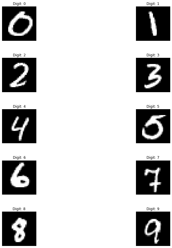
Let’s plot an image example for each possible class (i.e. digits from 0 to 9).
def get_random_element_with_label (data, lbls, lbl):
  """Returns one numpy array (one column) with an example of a choosen label."""

  tmp = lbls == lbl
  subset = data[tmp.flatten(), :]
  return subset[randint(0, subset.shape[0]), :]
# The following line is needed to reshape the training dataset
# (to plot some image examples)
input_example = input_train.reshape(60000, 784)
# The following code create a numpy array where in column 0 you will find
# an example of label 0, in column 1 of label 1 and so on.
labels_overview = np.empty([784, 10])
for i in range (0, 10):
    col = get_random_element_with_label(input_example, target_train, i)
    labels_overview[:,i] = col
f = plt.figure(figsize = (15, 15))
count = 1
for i in range(0, 10):
  plt.gray()
  plt.subplot(5, 2, count)
  count = count + 1
  plt.subplots_adjust(hspace = 0.5)
  plt.title('Digit: ' + str(i))
  some_digit_image = labels_overview[:, i]
  plt.imshow(some_digit_image.reshape(28, 28))
  plt.axis('off')
  pass
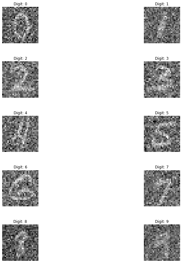
Adding Noise to the Dataset
We know add a source of noise to the MNIST images (by means of np.random.normal function), since our objective will be to remove the same noise from them.
noise_factor = 0.55
pure = input_train
pure_test = input_test
noise = np.random.normal(0, 1, pure.shape)
noise_test = np.random.normal(0, 1, pure_test.shape)
noisy_input = pure + noise_factor * noise
noisy_input_test = pure_test + noise_factor * noise_test
Now, let’s plot some examples of images corrupted by noise (one for each class, as in the figure above).
# The following line is needed to reshape the training dataset
# (to plot some image examples)
input_example_noise = noisy_input.reshape(60000, 784)
# The following code create a numpy array where in column 0 you will find
# an example of label 0, in column 1 of label 1 and so on.
labels_overview = np.empty([784, 10])
for i in range (0, 10):
    col = get_random_element_with_label(input_example_noise, target_train, i)
    labels_overview[:,i] = col
f = plt.figure(figsize = (15, 15))
count = 1
for i in range(0, 10):
  plt.gray()
  plt.subplot(5, 2, count)
  count = count + 1
  plt.subplots_adjust(hspace = 0.5)
  plt.title('Digit: ' + str(i))
  some_digit_image = labels_overview[:, i]
  plt.imshow(some_digit_image.reshape(28, 28))
  plt.axis('off')
  pass
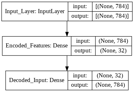
Autoencoder with Feed-Forward Neural Networks
Now we need to create the keras models. An autoencoder is made of two main parts: an encoder and a decoder. The function below create_autoencoders() returns the following parts as separate models:
the encoder
the decoder
the complete model, when the encoder and decoder are joined in one model.
def create_autoencoders(feature_layer_dim = 16):

  input_img = Input(shape = (784,), name = 'Input_Layer')
  # 784 is the total number of pixels of MNIST images

  # The layer encoded has a dimension equal to feature_layer_dim and contains
  # the encoded input (therefore the name)
  encoded = Dense(feature_layer_dim, activation = 'relu', name = 'Encoded_Features')(input_img)
  decoded = Dense(784, activation = 'sigmoid', name = 'Decoded_Input')(encoded)

  autoencoder = Model(input_img, decoded)
  encoder = Model(input_img, encoded)

  encoded_input = Input(shape = (feature_layer_dim,))
  decoder = autoencoder.layers[-1]
  decoder = Model(encoded_input, decoder(encoded_input))

  return autoencoder, encoder, decoder
# 32 is the number of latent features of our autoencoder
autoencoder, encoder, decoder = create_autoencoders(32)
autoencoder.summary()
Model: "model"
_________________________________________________________________
Layer (type)                 Output Shape              Param #
=================================================================
Input_Layer (InputLayer)     [(None, 784)]             0
_________________________________________________________________
Encoded_Features (Dense)     (None, 32)                25120
_________________________________________________________________
Decoded_Input (Dense)        (None, 784)               25872
=================================================================
Total params: 50,992
Trainable params: 50,992
Non-trainable params: 0
_________________________________________________________________
plot_model(autoencoder, show_shapes = True)
As for any Keras model we need to compile the model and then fit it to the data. As you can see we don’t need any custom code to work with autoencoders. A simple model definition \(\rightarrow\) compile \(\rightarrow\) fit is enough.
# Model configuration
batch_size = 150
no_epochs = 30
validation_split = 0.2
# Compile and fit data
autoencoder.compile(optimizer = 'adam', loss = 'binary_crossentropy')
autoencoder.fit(noisy_input, pure,
                epochs = no_epochs,
                batch_size = batch_size,
                validation_split = validation_split)
Epoch 1/30
320/320 [==============================] - 4s 4ms/step - loss: 0.3580 - val_loss: 0.1933
Epoch 2/30
320/320 [==============================] - 1s 3ms/step - loss: 0.1852 - val_loss: 0.1655
Epoch 3/30
320/320 [==============================] - 1s 3ms/step - loss: 0.1612 - val_loss: 0.1519
Epoch 4/30
320/320 [==============================] - 1s 3ms/step - loss: 0.1492 - val_loss: 0.1445
Epoch 5/30
320/320 [==============================] - 1s 3ms/step - loss: 0.1424 - val_loss: 0.1397
Epoch 6/30
320/320 [==============================] - 1s 3ms/step - loss: 0.1372 - val_loss: 0.1365
Epoch 7/30
320/320 [==============================] - 1s 3ms/step - loss: 0.1340 - val_loss: 0.1343
Epoch 8/30
320/320 [==============================] - 1s 3ms/step - loss: 0.1322 - val_loss: 0.1327
Epoch 9/30
320/320 [==============================] - 1s 3ms/step - loss: 0.1306 - val_loss: 0.1319
Epoch 10/30
320/320 [==============================] - 1s 3ms/step - loss: 0.1299 - val_loss: 0.1316
Epoch 11/30
320/320 [==============================] - 1s 3ms/step - loss: 0.1293 - val_loss: 0.1310
Epoch 12/30
320/320 [==============================] - 1s 3ms/step - loss: 0.1288 - val_loss: 0.1310
Epoch 13/30
320/320 [==============================] - 1s 3ms/step - loss: 0.1290 - val_loss: 0.1307
Epoch 14/30
320/320 [==============================] - 1s 3ms/step - loss: 0.1284 - val_loss: 0.1306
Epoch 15/30
320/320 [==============================] - 1s 3ms/step - loss: 0.1286 - val_loss: 0.1304
Epoch 16/30
320/320 [==============================] - 1s 3ms/step - loss: 0.1285 - val_loss: 0.1304
Epoch 17/30
320/320 [==============================] - 1s 3ms/step - loss: 0.1287 - val_loss: 0.1303
Epoch 18/30
320/320 [==============================] - 1s 3ms/step - loss: 0.1284 - val_loss: 0.1303
Epoch 19/30
320/320 [==============================] - 1s 3ms/step - loss: 0.1284 - val_loss: 0.1303
Epoch 20/30
320/320 [==============================] - 1s 3ms/step - loss: 0.1283 - val_loss: 0.1302
Epoch 21/30
320/320 [==============================] - 1s 3ms/step - loss: 0.1281 - val_loss: 0.1302
Epoch 22/30
320/320 [==============================] - 1s 3ms/step - loss: 0.1282 - val_loss: 0.1303
Epoch 23/30
320/320 [==============================] - 1s 3ms/step - loss: 0.1279 - val_loss: 0.1301
Epoch 24/30
320/320 [==============================] - 1s 3ms/step - loss: 0.1278 - val_loss: 0.1302
Epoch 25/30
320/320 [==============================] - 1s 3ms/step - loss: 0.1281 - val_loss: 0.1301
Epoch 26/30
320/320 [==============================] - 1s 3ms/step - loss: 0.1281 - val_loss: 0.1302
Epoch 27/30
320/320 [==============================] - 1s 3ms/step - loss: 0.1281 - val_loss: 0.1301
Epoch 28/30
320/320 [==============================] - 1s 3ms/step - loss: 0.1282 - val_loss: 0.1303
Epoch 29/30
320/320 [==============================] - 1s 3ms/step - loss: 0.1278 - val_loss: 0.1301
Epoch 30/30
320/320 [==============================] - 1s 3ms/step - loss: 0.1281 - val_loss: 0.1301
<tensorflow.python.keras.callbacks.History at 0x7f91f0304cd0>
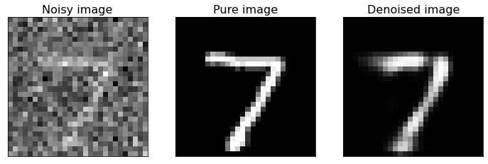
Examples of Denoised Images
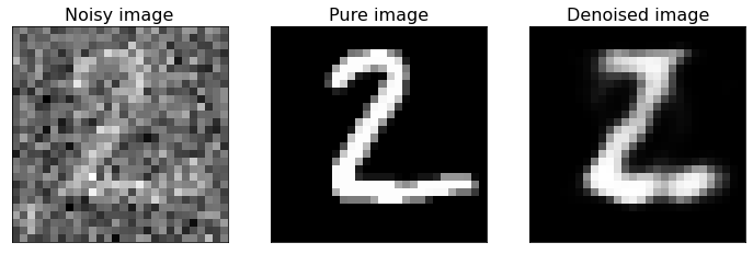
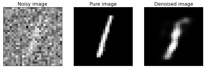
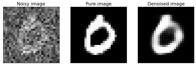
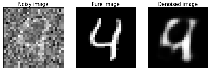
Now we plot some examples of denoised images, comparing them with the original pure images, to see how well the built autoencoder behaves.
# Generate denoised images
number_of_visualizations = 6
samples = noisy_input_test[:number_of_visualizations]
targets = target_test[:number_of_visualizations]
denoised_images = autoencoder.predict(samples)
# Plot denoised images
for i in range(0, number_of_visualizations):
  plt.gray()
  # Get the sample and the reconstruction
  noisy_image = noisy_input_test[i].reshape(28, 28)
  pure_image  = pure_test[i].reshape(28, 28)
  denoised_image = denoised_images[i].reshape(28, 28)
  input_class = targets[i]
  # Matplotlib preparations
  fig, axes = plt.subplots(1, 3)
  fig.set_size_inches(12, 7)
  # Plot sample and reconstruciton
  axes[0].imshow(noisy_image)
  axes[0].set_title('Noisy image', fontsize = 16)
  axes[0].get_xaxis().set_visible(False)
  axes[0].get_yaxis().set_visible(False)
  axes[1].imshow(pure_image)
  axes[1].set_title('Pure image', fontsize = 16)
  axes[1].get_xaxis().set_visible(False)
  axes[1].get_yaxis().set_visible(False)
  axes[2].imshow(denoised_image)
  axes[2].set_title('Denoised image', fontsize = 16)
  axes[2].get_xaxis().set_visible(False)
  axes[2].get_yaxis().set_visible(False)
  plt.show()
<Figure size 432x288 with 0 Axes>
<Figure size 432x288 with 0 Axes>
<Figure size 432x288 with 0 Axes>
<Figure size 432x288 with 0 Axes>
<Figure size 432x288 with 0 Axes>
<Figure size 432x288 with 0 Axes>
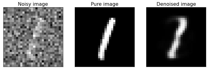
As you can see from the above figure, the model we built can reconstruct the original version of noisy digit images. If you have new noisy images of the same type you can apply the model to them and de-noise the same images.
If you compare this last figure with the last figure of Denoising_autoencoders_with_CNN.ipynb notebook, you can notice that CNNs are better suited to this kind of task. In fact, they are specifically designed for working with images, more than FFNNs.