Introduction
Deep learning is based on large and complex networks made of large number of simple computational units. Companies on the fore front of research are dealing with networks with 160 billion of parameters. To put things in perspective this number is half of the number of the stars in our galaxy, or 1.5 times the number of people that ever lived. On a basic level, neural networks are a large set of differently interconnected units each performing a specific (and usually relatively easy) computation. They remind of the game LEGO where you can build very complex things using very simple and basic units. Neural networks are similar. Using relatively simple computational units you can build very complex systems. We can vary the basic units changing how they compute the result, how they are connected to each other, how they use the input values and so on. Roughly formulated all those aspects define what is known as the network architecture. Changing it, will change how the network learn, how good the predictions are and so on.
Those basic units are known, due to a biological parallel with the brain, as neurons. Each neuron does basically a very simple thing: take a certain number of inputs (real numbers) and calculates an output (also a real number). Our inputs will be indicated in this book with \(x_i\) (real numbers) with \(i=1,2,…,n_x\), where \(i\) is an integer and \(n_x\) is the number of input attributes (often called features). As an example of input features, you can imagine the age and weight of person (so we would have \(n_x=2\)). \(x_1\) could be the age and \(x_2\) could be the weight. In real life the number of features can be easily very big.
In a more mathematical form, given \(n_x\) real parameters \(w_i\) (with \(i=1,2,…,n_x\)) and a constant \(b\) (usually called bias), the neuron will calculate first what is usually indicated in literature and in books with \(z\):
it will then apply a function \(f\) to \(z\), giving the output \(\hat y\)
Computational Graph
One single neuron can be depicted as a computational graph. You can check the book for more details on this. But in general one neuron can be visualised as in Fig. 1
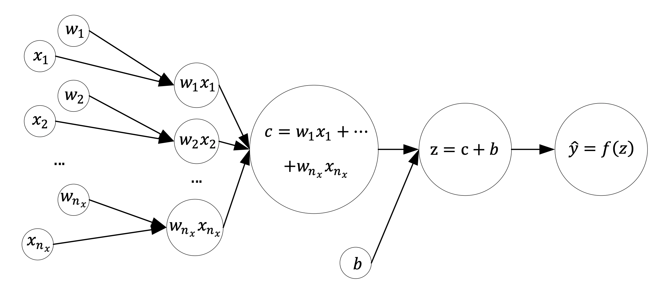
Fig. 1 one neuron computational Graph.
In Fig. 1 we have the following notation
\(w_i\) are the weights
\(x_i\) are the inputs (for example the pixel values of an image)
\(b\) is the so called bias
\(f()\) is the activation functions
This is a very general way of building the computational graph for one single neuron. In general in books and blogs you will find this more compact form
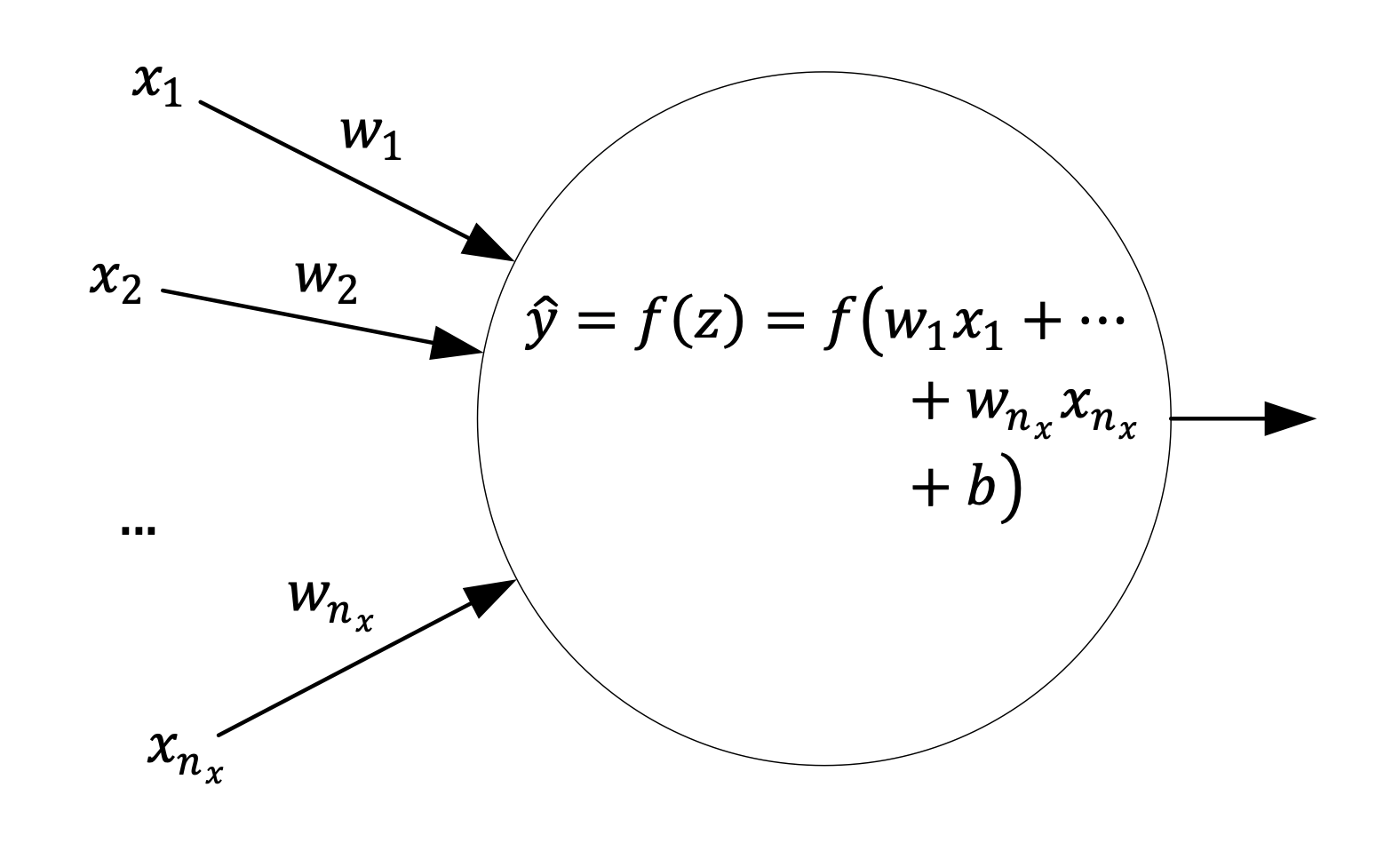
Fig. 2 one neuron computational Graph. This form is more compact and is typically found in blogs and books.
Or in an even more simple form

Building one neuron in Keras
In the next chapters you will see many examples on how you can choose the activation function and the loss function to solve different problems, namely linear regression and logistic regression. In Keras to build a network with one single neuron is really simple and can be done with
model = keras.Sequential([
   layers.Dense(1, input_shape = [...])
])
In the next chapters you will see many complete examples on how to do that.